In previous articles we covered ESEDatabaseView for raw database exploration, and SrumECmd for fast command-line parsing.

This article introduces a fourth approach: SRUM-DUMP v3.

Version 3 is a significant redesign from 2.6.

If you waana learn or see how version 2.6 works Check out below article

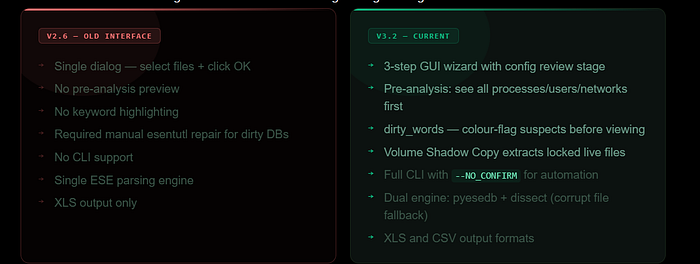
The old single-dialog interface is gone. In its place is a three-step GUI wizard, a JSON configuration system, a "dirty words" feature for keyword highlighting, built-in Volume Shadow Copy support for locked live-system files, and full command-line support for automated workflows.

If you used the old version and haven't upgraded, the new interface looks entirely different.

— — — — — — — — — — — — — — — — — — — — — — — — — — — — — — — — — — — — — —

Section 1 — What Changed from 2.6 to 3.2

The 2.6 interface was a single dialog — you selected files, clicked OK, and got a spreadsheet. Fast and simple, but no opportunity to guide the analysis.

Version 3 rebuilds the workflow around a three-step process that adds two important new concepts: the configuration file and dirty words.

The configuration file (srum_dump_config.json) is generated after the tool's first pass through the database. It lists every process path, user SID, and network interface found — before the full analysis runs. This lets you see exactly what's in the database before committing to the full extraction. You can rename entries to be more readable, and flag specific strings for highlighting.

The dirty words feature lets you define keywords that will be colour-coded in the output. Any string matching cmd.exe, powershell.exe, a specific malware filename, a suspect username, or a suspicious network name will be highlighted in the colour you specify. This means when you open the output spreadsheet, your points of interest are already visually flagged — you don't have to manually scan thousands of rows.

The biggest operational change is locked file handling. SRUM-DUMP 3 can extract SRUDB.dat from a live system through Volume Shadow Copies without requiring manual esentutl repair first. And if the database is corrupt, there are now two ESE parsing engines to try — pyesedb and dissect — and switching between them is a single flag change.

— — — — — — — — — — — — — — — — — — — — — — — — — — — — — — — — — — — — — —

Section 2 — The Three-Step GUI Wizard

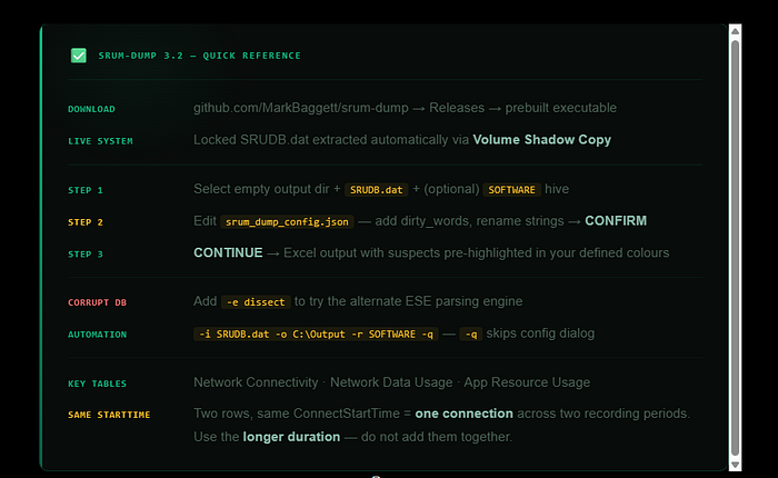
Download the prebuilt executable from the Releases page at github.com/MarkBaggett/srum-dump. No installation is required — just run the executable. The interface opens on a three-step wizard.

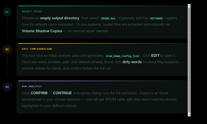
Step 1 is file selection. You choose an empty output directory first,

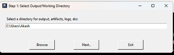
then select SRUDB.dat.

On a live system you'll find it at C:\Windows\System32\sru\srudb.dat and administrative privileges are required.

If those files are locked by the OS — which is normal on a running system — SRUM-DUMP will extract them through Volume Shadow Copies automatically.

You don't need to manually copy or repair the database first. You can also optionally provide the SOFTWARE registry hive, which enables automatic resolution of interface LUIDs to human-readable SSID network names.

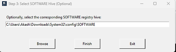
Step 2 is configuration review. After the initial analysis pass, the tool generates srum_dump_config.json and opens it for editing.

This is where SRUM-DUMP v3 fundamentally differs from version 2.6. Before the full extraction runs, you can see every process, user, and network in the database.

You can rename entries to make them more readable, and you can define dirty words to highlight during analysis.

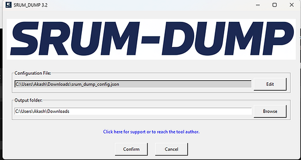
Step 3 is execution. Click Confirm, then Continue. A progress dialog appears and the Close button is disabled until the analysis completes.

The output — an Excel spreadsheet with one tab per SRUM table — is written to your output directory.

Open it and your dirty word matches are already highlighted in the colours you defined.

— — — — — — — — — — — — — — — — — — — — — — — — — — — — — — — — — — — — — —

Section 3 — The Configuration File and dirty_words

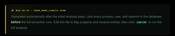
The configuration file is the most powerful new feature in version 3. It's generated automatically after the first analysis pass and saved as srum_dump_config.json in your output directory.

Think of it as a manifest — before the full extraction runs

SRUM-DUMP has already identified every process path, user SID, and network interface in the database and listed them here.

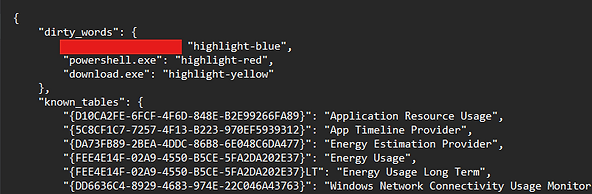
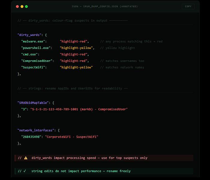
The dirty_words section is where you define keywords to colour-highlight in the output. Any string you add — a process name, a username, a network name — will be changed to the specified colour wherever it appears in the spreadsheet.

"dirty_words": {
    "cmd.exe": "highlight-red",
    "powershell.exe": "highlight-yellow",
    "suspicious_process": "general-red-bold"
}

Available colours include highlight-red, highlight-yellow, and general-red-bold. Note that dirty words do have a processing cost — adding many of them will increase analysis time. Use them for your top suspects rather than broad filters.

The strings section is also editable. Each AppID and UserID in the database is listed with its resolved string. If you know the username behind a SID, or want to flag a network with a label like "SuspectWifi", you can modify the strings here before the final run. String modifications don't carry the same performance cost as dirty words, so use them freely.

A practical workflow:

after the initial pass generates the config file, scan the process list for anything unusual before adding dirty words. If you're looking for a specific piece of malware, add its filename. If you know a suspect username, add that. If a particular network is under scrutiny, add that too. Then run the full analysis — the output will have your suspects pre-highlighted, saving significant manual review time on large datasets.

— — — — — — — — — — — — — — — — — — — — — — — — — — — — — — — — — — — — — —

Section 4 — Command-Line Usage

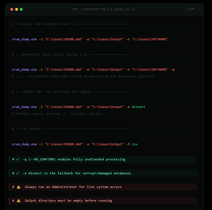
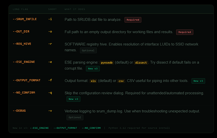
SRUM-DUMP 3 includes full command-line support, making it suitable for scripted workflows, automated collection pipelines, and integration with tools like KAPE. Every option available in the GUI is also available as a CLI flag.

• The — NO_CONFIRM flag (-q) skips the configuration review dialog, which is what you want for automated processing.
• The — ESE_ENGINE flag is particularly useful when dealing with corrupt databases — if the default pyesedb engine fails or produces incomplete output, switching to dissect sometimes recovers data the other engine cannot.
• The — OUTPUT_FORMAT flag lets you choose CSV instead of XLS, which is useful when piping output into other tools.

All flags use double-dash for long form and single-dash for short form.

• The input file flag is — SRUM_INFILE or -i. Output directory is — OUT_DIR or -o.

— — — — — — — — — — — — — — — — — — — — — — — — — — — — — — — — — — — — — —

Section 5 — Reading the Output: Three Key Tables

The Excel spreadsheet output contains one tab per SRUM table. The three most important for investigation are Network Connectivity Usage, Network Data Usage, and Application Resource Usage.

Network Connectivity Usage

The Network Connectivity Usage table documents when the system connected to each network, how long each connection lasted, and which wireless interface was used. This is one of the best tables for establishing the physical location of a computer during a given time window.

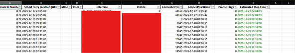
Each row represents a SRUM entry.

• The timestamp column shows when the SRUM entry was recorded — typically at each hour boundary.
• The network interface column tells you the protocol used — Wireless 802.11 for WiFi.
• The network name column shows the resolved SSID if a SOFTWARE hive was provided.
• The connected time column shows how long that network had been connected at the time of the SRUM entry.
• The connect start time column shows when the connection originally began.

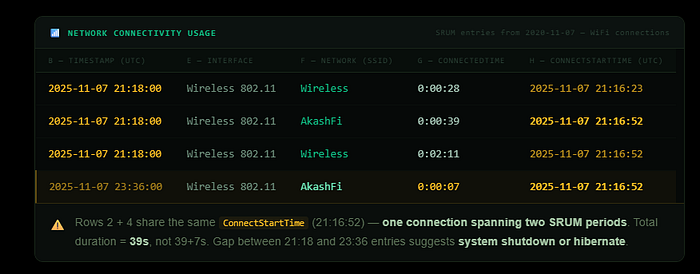
One important interpretation note: you will frequently see the same network appearing across two SRUM entries with the same ConnectStartTime. This is not two separate connections — it's a single connection spanning across two recording periods. When you see this pattern, take the ConnectStartTime as the beginning of the connection and the longest ConnectedTime value as the total duration. Adding the two time values together would overstate the connection length.

Additionally, if two consecutive SRUM entries are more than 60 minutes apart (plus or minus 10 minutes), a system shutdown or hibernate almost certainly occurred during that gap. SRUM entries are typically recorded every hour, so a gap larger than that is meaningful.

— — — — — — — — — — — — — — — — — — — — — — — — — — — — — — — — — — — — — —

Network Data Usage

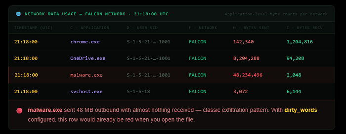
The Network Data Usage table records which specific applications were using each network during each SRUM recording period. Where the Connectivity table tells you which networks the system was connected to and when, this table tells you what was happening on those networks at the application level.

Each row shows an application path, the user SID responsible for running it, the network it communicated on, and the total bytes sent and received since the last SRUM entry. The application path is the full executable path, already resolved from AppID by the tool.

This table is particularly useful for identifying unusual data volumes. If you see a process transferring large amounts of data on a network that wouldn't normally have that traffic, or a process you wouldn't expect to be making network calls at all, those are your investigative leads. Filter by the AppId column to isolate specific applications across all recording periods and see their full network activity history.

One precision note:

the byte counts represent raw data at the protocol level and include protocol overhead and compressed data. They may not match exactly to a file size you're trying to account for, but they are reliable for identifying relative volumes and patterns.

— — — — — — — — — — — — — — — — — — — — — — — — — — — — — — — — — — —

Application Resource Usage

The Application Resource Usage table is the broadest of the three — it records all applications active during each SRUM recording period, not just those using the network. This makes it the primary table for evidence of application execution.

Each row records the full executable path, the user SID, the volume and directory, CPU cycle time for foreground and background processing, memory working set size, and foreground and background bytes read and written to disk. The timestamp represents the end of the 60-minute window during which that application was active.

For a forensic analyst, the most immediately useful fields are the application path, the user SID, and the timestamp. Together these establish what ran, under whose account, and during what hour. Cross-referencing with the Network Data Usage table for the same time window shows whether that application was also making network connections.

The CPU and disk I/O fields require more research before they can be relied upon for definitive conclusions — the forensic community is still developing best practices for interpreting them. The execution evidence they provide, however, is solid.

— — — — — — — — — — — — — — — — — — — — — — — — — — — — — — — — — — — — — —

Conclusion + Quick Reference

SRUM-DUMP 3 takes what was already a capable forensic tool and adds the investigative workflow it was always missing. The configuration file gives you a preview of what's in the database before you commit to the full extraction. Dirty words mean your suspects are flagged before you open the spreadsheet. Volume Shadow Copy support removes the manual locked-file problem from the process entirely.

The three key tables remain the same as in version 2.6 — Network Connectivity Usage for location and connection timeline, Network Data Usage for application-level bandwidth and exfiltration indicators, and Application Resource Usage for comprehensive execution evidence.

SRUM-DUMP is available free.

It is the fourth tool in this series covering SRUM analysis, alongside ESEDatabaseView, SrumECmd, and the broader raw database exploration approaches documented in earlier articles.

— — — — — — — — — — — — — — — — — Dean — — — — — — — — — — — — — — — — — —

Check Out series Link below: