Reinforcement Learning Through Energy Landscapes: A Visual, Intuitive Understanding of How…

When people first encounter Reinforcement Learning (RL), they are introduced to a wall of unfamiliar terminology:

States
Actions
Policies
Value Functions
Bellman Equations
Q-Tables

While these concepts are important, they often hide the most intuitive picture.

At its core, Reinforcement Learning can be viewed as a journey through an energy landscape.

Imagine placing a marble on a mountainous terrain.

The marble wants to roll toward lower energy regions.

An RL agent does something similar.

It explores a landscape of possible behaviors and gradually discovers pathways that lead to higher rewards.

Once you start viewing RL this way, many famous algorithms become surprisingly easy to understand.

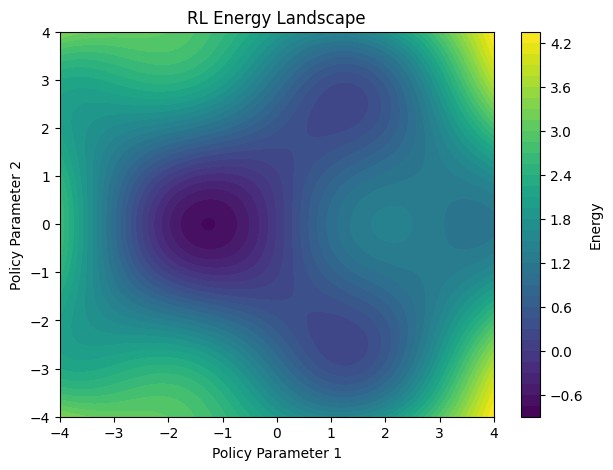
The Energy Landscape

Consider a landscape:

Each point represents a policy.

A policy is simply:

which means:

"Given state s, choose action a."

Some policies are poor.

Some are excellent.

The goal of RL is finding the highest-performing policy.

In optimization language:

where:

is the expected reward.

Visualizing the Landscape

Imagine a surface:

Low energy:

High reward

High energy:

Poor reward

Now learning becomes:

Bad Policy
      ↓
Exploration
      ↓
Better Policy
      ↓
Optimal Policy

Bad Policy
      ↓
Exploration
      ↓
Better Policy
      ↓
Optimal Policy

The agent is navigating a rugged terrain.

Random Search: Wandering Blindly

The simplest strategy is random exploration.

Imagine a hiker moving without a map.

import numpy as np
position = np.random.randn(2)
for step in range(100):
    position += 0.1*np.random.randn(2)

import numpy as np
position = np.random.randn(2)
for step in range(100):
    position += 0.1*np.random.randn(2)

The trajectory looks chaotic.

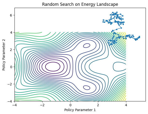
Eventually the hiker may discover a valley.

But it is inefficient.

Q-Learning: Building a Terrain Map

Q-Learning does something smarter.

Instead of wandering blindly, it builds a memory of the landscape.

The famous update rule:

means:

Update your estimate using what you learned from the future.

Over time:

Unknown Terrain
      ↓
Partial Map
      ↓
Accurate Map

Unknown Terrain
      ↓
Partial Map
      ↓
Accurate Map

The agent learns where the valleys are.

Gradient-Based Policy Learning

Now imagine the hiker can feel the slope beneath their feet.

Instead of moving randomly:

← downhill

← downhill

they follow gradients.

Policy Gradient methods optimize:

using:

This is equivalent to descending an energy surface.

REINFORCE: Following the Slope

REINFORCE estimates:

Interpretation:

If an action produced good rewards:

Do more of it

Do more of it

If rewards were poor:

Do less of it

Do less of it

The landscape begins guiding the agent.

Actor-Critic: Explorer + Guide

Actor-Critic splits learning into two agents.

Actor

Moves through the terrain.

Critic

Estimates landscape elevation.

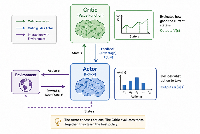
The Actor explores.

The Critic evaluates.

Together they navigate much more efficiently.

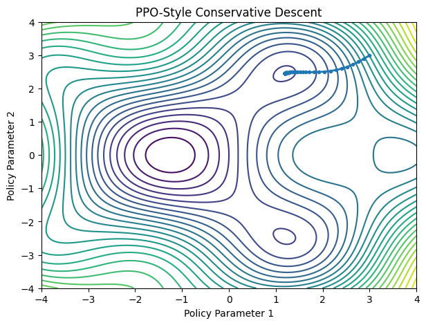
PPO: Safe Mountain Climbing

One problem with gradients:

Sometimes the agent jumps too far.

Valley
  ↓
JUMP!

Falls off cliff

Valley
  ↓
JUMP!

Falls off cliff

PPO (Proximal Policy Optimization) introduces a trust region.

Objective:

Meaning:

Improve, but don't change too much at once.

PPO became one of the most widely used RL algorithms because it balances exploration and stability.

SAC: Adding Temperature

Soft Actor Critic introduces entropy.

Objective:

where:

is entropy.

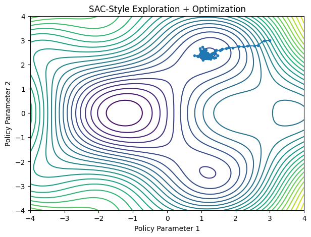
Interpretation:

Reward
+
Curiosity

Reward
+
Curiosity

The agent doesn't merely seek the deepest valley.

It also prefers landscapes with multiple promising paths.

This prevents premature convergence.

Creating the Landscape Visualization

Generate a synthetic reward surface:

import numpy as np

x = np.linspace(-4,4,200)
y = np.linspace(-4,4,200)
X,Y = np.meshgrid(x,y)
Z = (
    np.sin(X)
    * np.cos(Y)
    + 0.1*(X**2 + Y**2)
)

import numpy as np

x = np.linspace(-4,4,200)
y = np.linspace(-4,4,200)
X,Y = np.meshgrid(x,y)
Z = (
    np.sin(X)
    * np.cos(Y)
    + 0.1*(X**2 + Y**2)
)

Visualize:

import matplotlib.pyplot as plt

plt.figure(figsize=(8,6))
plt.contourf(X,Y,Z,levels=50)
plt.colorbar()
plt.title("Policy Energy Landscape")
plt.show()

import matplotlib.pyplot as plt

plt.figure(figsize=(8,6))
plt.contourf(X,Y,Z,levels=50)
plt.colorbar()
plt.title("Policy Energy Landscape")
plt.show()

Simulating Different Algorithms

Random Search:

path = [np.array([0,0])]
for _ in range(200):
    path.append(
        path[-1]
        + 0.2*np.random.randn(2)
    )

path = [np.array([0,0])]
for _ in range(200):
    path.append(
        path[-1]
        + 0.2*np.random.randn(2)
    )

Gradient Descent:

for _ in range(100):
gradx = ...
    grady = ...
    x -= 0.1*gradx
    y -= 0.1*grady

for _ in range(100):
gradx = ...
    grady = ...
    x -= 0.1*gradx
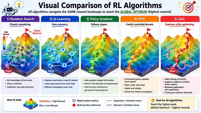
    y -= 0.1*grady

Overlay trajectories on the contour map.

The resulting figure immediately reveals:

Random Search wanders
Q-Learning explores then exploits
PPO descends carefully
SAC explores broader regions

Why This Perspective Matters

Energy landscapes unify ideas from:

Reinforcement Learning
Statistical Physics
Dynamical Systems
Optimization Theory
Deep Learning

Instead of memorizing equations, you can think:

Agent
   ↓
Explores Landscape
   ↓
Finds Better Valleys
   ↓
Learns Better Policies

Agent
   ↓
Explores Landscape
   ↓
Finds Better Valleys
   ↓
Learns Better Policies

The mathematics becomes a description of movement through that landscape.

And suddenly, Reinforcement Learning feels less like abstract equations and more like watching intelligence emerge from a journey through a complex terrain.

The next time you hear terms like PPO, SAC, or Actor-Critic, imagine a traveler crossing mountains, discovering valleys, and gradually learning the shape of an unseen world.

That is Reinforcement Learning.

Contents