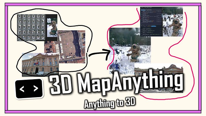
Have you ever wished you could just point your camera at something and instantly have a 3D model of it?

I've just finalized a workflow that does precisely that.

It turns any set of images, even blurry ones from an old smartphone, into a metric 3D point cloud.

I was digging through old travel photos and found a set from Bergen, Norway.

I'd snapped a few pictures of this cool troll statue, trying to do photogrammetry with my phone back in 2016.

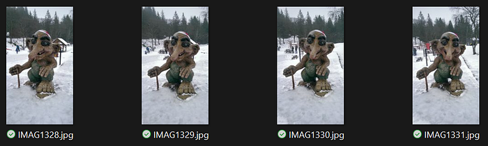
This time, I fed those same photos into a new AI model. In under a minute, I had a complete, scaled 3D model.

The lesson? The hardware isn't the bottleneck anymore; it's the intelligence of the software.

What if you didn't need a perfect capture process?

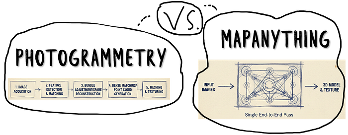
We're moving from "data-hungry" photogrammetry to "data-intelligent" reconstruction.

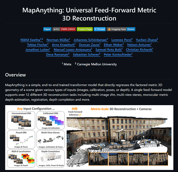
Instead of needing hundreds of perfect, overlapping photos, transformer-based AI like MapAnything understands the geometry within the images.

It's a hybrid approach — it feels like photogrammetry, but it thinks like an AI, inferring depth and shape from context, not just pixels.

This isn't just a cool trick.

It means you can generate 3D assets faster and from messier, more diverse data sources — like drone footage, Google Street View, or even AI-generated images.

In this tutorial, I'm going to walk you through the entire process, step-by-step.

🦚 Florent's Note: I've spent fifteen years in this field, from land surveyor to spatial AI professor. I've seen every technology promise to "revolutionize" 3D capture. Most failed. Transformers are different. They fundamentally understand spatial relationships much like humans do — through context, not just features.

The question then becomes: What would you build if creating 3D data was as easy as taking a photo?

🦚Florent Poux, Ph.D.: If you are new to my (3D) writing world, welcome! We are embarking on an exciting adventure that enables you to master a crucial 3D Python skill. Before diving, I like to establish a clear scenario, the mission brief.

Once the scene is laid out, we embark on the Python journey. Everything is given. You will see Tips (🌱Growing Notes, 📈Market Insights, and 🦥Geeky Notes), the code (Python), and 🗺️diagrams to help you get the most out of this article.

→ The download link for all the resources 📦 is at the end of the article. Thanks to the 3D Geodata Academy for their support of this endeavor.

Your Mission: Documenting Cultural Heritage in the Digital Age

You're standing in Bergen, Norway. Snow is misting the cobblestones. Tourists are clustering around the medieval wharf.

There's a troll statue here. Massive. Intricately carved. Part of the city's folklore identity.

The museum director approaches you. They need a digital archive. High-quality 3D model for virtual exhibits. Something visitors worldwide can explore. They want it accurate. They want it fast.

You have a smartphone and confidence in Python.

The old approach would involve specialists. Weeks of planning. Photogrammetry rigs. Manual calibration sessions. Dense point cloud processing. Mesh generation. Texture mapping.

Months of work. Tens of thousands in costs.

You walk around the troll instead. Thirty-four photos from different angles. Natural lighting. Handheld captures. No tripod. No reference targets.

Back at your laptop, you want to investigate a new approach: a transformer architecture called MapAnything.

What you want is a complete point cloud. RGB colors mapped from source images. Ready for Open3D visualization. Export to PLY for museum integration.

🦚 Florent's Note: You want a transformer that learns fundamental 3D geometry from massive datasets. That understands depth from parallax. That predicts normals from shading. That reasons about occlusion and visibility.

The director is waiting, and you want to make a good impression on him.

This is the workflow you're about to build. Zero-shot reconstruction means zero fine-tuning. The model never saw your troll statue during training. It doesn't need to.

So how do we actually structure this ambitious transformation?

Initialization: Setting Up Your Development Environment

Alright, let's ensure we approach the innovative method with a sound, step-by-step system design.

First, let us properly organize our data.

2D — 3D Dataset Access

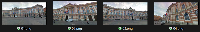
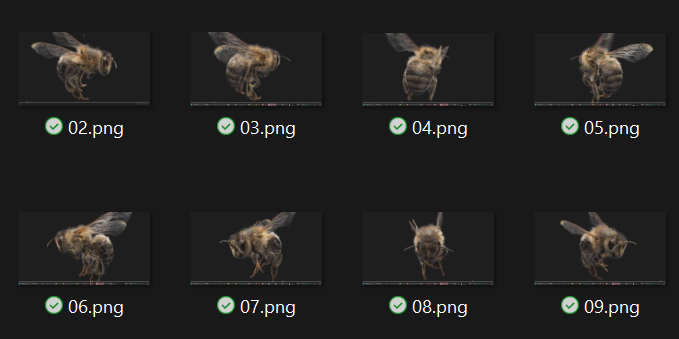
Use any dataset of your choice, or the one given to you at the end of the article. You can also retrieve random pictures from Google Street View, AI-generated images, or anything where you have multiple viewpoints of the same object / scene.

For example, I also conducted experiments using poor-quality street-view images from Google.

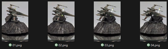
And even some screenshots I extracted from an X-Wing model in a short-form video (I cannot trace the original author; help me if you know who it is, so I can share the link to its short video!).

If using the Bergen troll images, you should have:

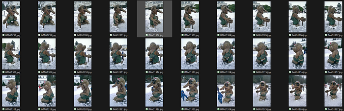
• Format: JPEG or PNG
• Resolution: 1520x2688 for each image
• Quantity: 34 images from varied viewpoints
• Coverage: Overlapping views essential for multi-view consistency

Place all images in a single folder (E.g. the DATA folder). We will handle loading automatically.

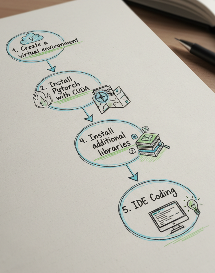
Beautiful! Now, we want first to ensure a proper data and environment setup. For that, we will proceed in 5 stages as illustrated below:

Creating a Clean Anaconda Environment

Open your terminal. Run these commands sequentially:

# Create new environment with Python 3.12
conda create -n anything python=3.12 -y
# Activate it
conda activate mapanything
# Verify version
python --version  # Should show Python 3.12.x

This isolates dependencies. Your system Python stays untouched.

🦚 Florent's Note: You need Python 3.12 to copy and paste the working solution. It may work with previous versions up to 3.10, but I haven't tested it.

Installing PyTorch with CUDA Support

This is where GPU capability enters. You must install PyTorch with CUDA bindings if you want to get great performances. Visit pytorch.org and select your configuration.

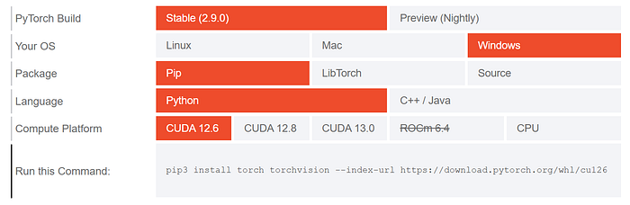
For CUDA 12.6 on Windows:

pip3 install torch torchvision --index-url https://download.pytorch.org/whl/cu126

To verify CUDA availability after installation, enter python (from the terminal, just type python), and then:

import torch
print(torch.cuda.is_available())  # Should return True
print(torch.cuda.get_device_name(0))  # Shows your GPU

CPU fallback exists, but expect 10–50x slower inference. Not practical for scaling.

Installing Libraries: MapAnything Framework

MapAnything lives on GitHub, not PyPI.

Install directly from source:

# Clone the repository
git clone https://github.com/facebookresearch/map-anything.git
cd map-anything

And then, install in editable mode. I recommend checking out the MapAnything Github Repo with all the instructions, super well done by the team!

# For all optional dependencies
# See pyproject.toml for more details
pip install -e ".[all]"
pre-commit install

The -e flag means "editable installation." Changes to source code reflect immediately without reinstalling.

Installing Other Libraries: Open3D + Numpy

Open3D will handle the point cloud geometry and rendering for our experiments. Hence it is optional, but useful when prototyping:

pip install open3d

Also, you'll need NumPy for array operations. Most installations include this automatically, but explicit is better than implicit:

pip install numpy

Finally, we can organize our project structure:

anything-project/
├── CODE/              # Your Python code, incl. map anything
├── DATA/              # Your input images, in subfolders
└── RESULTS/           # Your output point clouds

Place your thirty-four troll images in DATA/. We will handle folder paths or explicit image lists.

Common Installation Issues and Fixes

Okay, I ran into some issues when installing MapAnything, or CUDA. Here are some troubleshooting tips I noted to help you:

Problem: CUDA out of memory errors Solution: The environment variable in our code helps:

os.environ["PYTORCH_CUDA_ALLOC_CONF"] = "expandable_segments:True"

This enables dynamic memory expansion instead of pre-allocation. Critical for variable image sizes.

Problem: Open3D fails to import Solution: Check Python version first. Then verify no conflicting installations:

pip uninstall open3d
pip install open3d==0.18.0

Problem: MapAnything import fails Solution: Ensure you're in the activated conda environment:

conda activate mapanything
python -c "from mapanything.models import MapAnything"

If this fails, reinstall from source.

Problem: Slow inference on GPU Solution: Verify PyTorch sees your GPU:

import torch
print(torch.cuda.is_available())
print(torch.version.cuda)

If False, you installed CPU-only PyTorch. Reinstall with CUDA.

Memory Requirements

Expect these approximate requirements:

• RAM: 16GB minimum, 32GB comfortable
• VRAM: 8GB minimum for 34 images, 12GB+ ideal
• Storage: 10GB for model cache + datasets

If your GPU has less VRAM, enable memory_efficient_inference=True in step 4. This trades speed for capacity—up to 2000 views on 140GB GPUs according to Meta's documentation.

The foundation is solid. Time to build the reconstruction?

🐅Take Action: Before moving to the code, verify your setup works. Run python and import each library: torch, mapanything, open3d, numpy. If any fail, revisit the relevant installation step. A clean environment now saves hours of debugging later. Once everything imports successfully, you're ready for the step-by-step workflow where we'll transform those troll photos into precise 3D geometry.

For deeper understanding of 3D reconstruction pipelines, photogrammetry workflows, and production-grade spatial systems, explore the 3D Reconstructor OS at learngeodata.eu — the complete professional track covering everything from 3D capture to 3D Digital Experience Delivery.

Configuring Memory Management and Core Imports

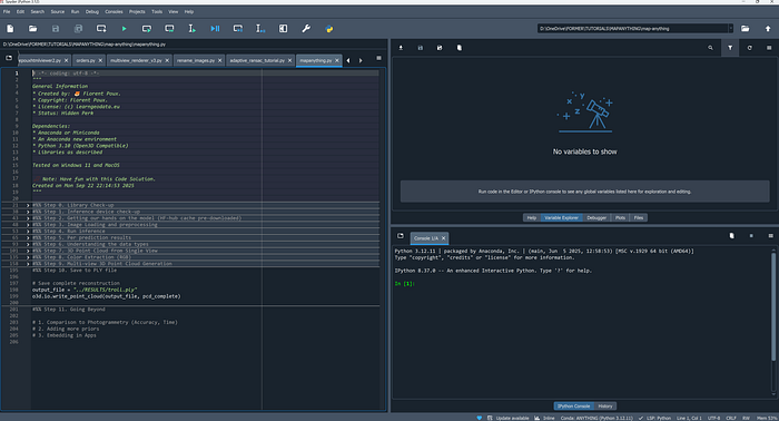
Allright, I assume you have everything set up, and comfortably installed with your IDE opened like me:

Let us make sure that we can use everything as planned in our 3D Python session.

PyTorch's default memory allocator pre-reserves CUDA memory in fixed blocks. This works beautifully for consistent workloads. Fails catastrophically for variable-sized inputs.

Your thirty-four troll images aren't uniform. Some capture wide angles. Others zoom into details. Resolution varies. Aspect ratios differ.

Each image generates a unique 3D prediction tensor. Fixed memory blocks fragment fast. You get "CUDA out of memory" errors despite having available VRAM.

The solution lives in one environment variable:

# Optional config for better memory efficiency
import os
os.environ["PYTORCH_CUDA_ALLOC_CONF"] = "expandable_segments:True"

This enables dynamic memory expansion. PyTorch requests CUDA memory as needed instead of pre-allocating pools. Memory fragmentation drops. Multi-view inference becomes stable.

🦚 Florent's Note: I discovered this setting the hard way during a 200-image reconstruction of a medieval church. Standard allocation failed at image 47. Enabling expandable segments processed all 200 without issues. The performance hit? Negligible — about 3% slower, but actually completes instead of crashing.

Right after memory configuration, we import the core libraries. PyTorch provides the tensor operations.

# For getting Pytorch
import torch

#For getting mapanything
from mapanything.models import MapAnything
from mapanything.utils.image import load_images

# Our base loving stack
import numpy as np
import open3d as o3d

MapAnything delivers the inference model. Open3D handles 3D visualization. NumPy manages array conversions. The order of imports matters less than their presence. Verify each load without errors before proceeding.

🦥 Geeky Note: The expandable_segments parameter was introduced in PyTorch 2.0. Earlier versions used max_split_size_mb for memory management, but it's less effective for transformer workloads. If you're on PyTorch 1.x, upgrade immediately—transformers demand modern memory strategies.

Understanding PyTorch's CUDA Context

When you import PyTorch, it doesn't immediately claim GPU memory.

CUDA context initializes lazily. First tensor operation to GPU triggers memory allocation.

This matters because errors appear during inference, not import. Your environment might look perfect until the model tries to create its first activation tensor.

Test CUDA availability explicitly in the next step instead of assuming imports succeeded.

But what device are we actually computing on?

Step 1: Device Detection and Hardware Verification

MapAnything is computationally intensive.

Each image generates roughly 3 million 3D predictions. Thirty-four images: 102 million points. The transformer processes these through multiple attention layers, each requiring matrix multiplications across high-dimensional embeddings.

CPU inference exists. It's technically functional. Practically unusable.

A single image takes 5–10 minutes on modern CPUs. Thirty-four images: 3–6 hours minimum. GPU inference? The same workload completes in 15–20 minutes.

The 20x speedup isn't a luxury. It's the difference between iterative experimentation and single-shot hoping.

device = "cuda" if torch.cuda.is_available() else "cpu"
print(device)

This code runs immediately. It tells you what hardware will execute inference.

If output shows "cuda": You're ready. Proceed confidently.

If output shows "cpu": Inference will work but be painfully slow. Consider cloud GPUs (Google Colab, AWS, Lambda Labs) or reduce image count for testing.

🌱 Growing Note: For production systems, add device capability checks beyond just availability. Query VRAM with torch.cuda.get_device_properties(0).total_memory and compare against your dataset requirements. For 34 images at 1920x1080, expect ~8GB VRAM usage. If you have less, enable memory-efficient inference in Step 4.

The device check gives you hardware confidence. Next, we need the intelligence — the pre-trained transformer model.

Step 2: Loading the MapAnything Model from HuggingFace Hub

This step downloads 1.2GB of learned spatial understanding.

Meta trained MapAnything on massive multi-view datasets. The model saw millions of image pairs. It learned how objects look from different angles.

It internalized the camera perspective geometry. It encoded depth cues from shading, texture, and parallax.

You're not training anything. You're loading that accumulated knowledge.

model = MapAnything.from_pretrained("facebook/map-anything").to(device)
# For Apache 2.0 license model, use "facebook/map-anything-apache"

The from_pretrained() method handles everything. First invocation downloads weights from HuggingFace Hub. Subsequent runs load from cache at ~/.cache/huggingface/.

The .to(device) call moves the model to GPU. This copies all 600 million parameters from CPU RAM to VRAM. Takes 3-5 seconds on modern hardware.

🦚 Florent's Note: License matters here. The default facebook/map-anything uses CC-BY-NC—free for research and education, restricted for commercial use. If you're building a paid service, use facebook/map-anything-apache instead. Performance is identical. Legal implications are not.

The Transformer Architecture Powering MapAnything

MapAnything builds on DUSt3R's encoder-decoder transformer architecture.

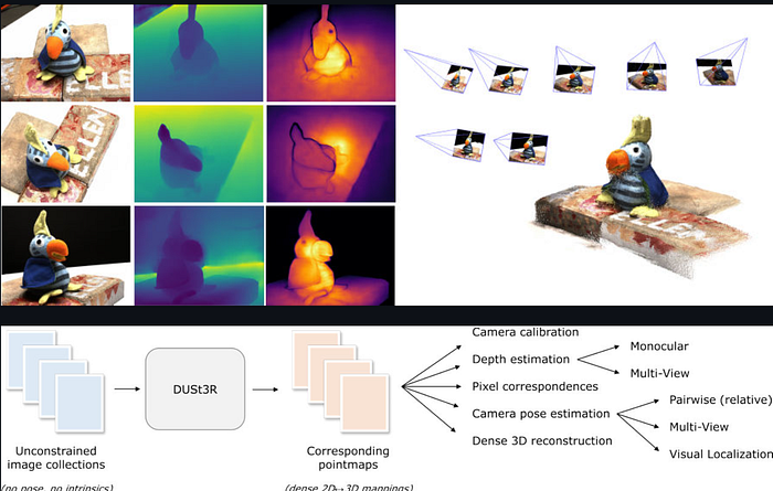
The encoder processes each image independently through a Vision Transformer (ViT). Patches of pixels become tokens. Self-attention discovers local and global features. No convolutional layers — pure attention mechanisms.

The decoder performs cross-attention between image pairs. It finds correspondences. It predicts dense 3D coordinates for every pixel. It estimates camera poses simultaneously.

This differs fundamentally from traditional photogrammetry. Classical pipelines:

1. Extract sparse features (SIFT, ORB)
2. Match features across views
3. Triangulate 3D points
4. Optimize bundle adjustment
5. Densify with multi-view stereo

MapAnything replaces all five steps with one forward pass. The transformer learned end-to-end geometry prediction.

The original paper is here: MapAnything: Scaling Dense Matching for General Cameras and Scenes (Meta AI Research, 2025). Please read it for the mathematical foundations of their loss functions and training procedures.

🦥 Geeky Note: MapAnything uses a hybrid attention mechanism — windowed self-attention for efficiency within images, then global cross-attention between pairs. This balances computational cost (O(n²) for global attention) with modeling power. For 34 images, the framework intelligently batches pairs to avoid computing all 561 possible combinations.

Model loaded. Device verified. Now we need data — the images that become geometry.

Step 3: Image Loading and Automatic Preprocessing

MapAnything accepts two input formats.

Option 1: Folder path — Point to directory containing images. The loader finds all JPEGs and PNGs automatically. Alphabetical ordering determines sequence.

Option 2: Explicit list — Provide Python list of full paths. Gives precise control over image order and selection.

For thirty-four troll images in ../DATA/, folder path is cleanest:

images = "../DATA/"  # or ["path/to/img1.jpg", "path/to/img2.jpg", ...]
views = load_images(images)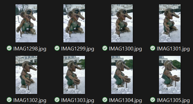

The load_images() function does substantial work behind the scenes.

• Resizing: Images scale to efficient resolutions. MapAnything handles various sizes, but standardizing to 1024x768 or similar improves batch processing. The function preserves aspect ratios while targeting manageable dimensions.
• Normalization: Pixel values convert from [0, 255] integers to ImageNet-standardized floats. Mean subtraction and standard deviation division ensure the model sees data matching its training distribution.
• Tensor conversion: NumPy arrays become PyTorch tensors. Channels reorder from HWC (height, width, channels) to CHW (channels, height, width) — PyTorch's expected format.
• Batching: Multiple images stack into a single tensor for efficient GPU processing.

You don't write this preprocessing. The framework handles it. You just point at images.

🌱 Growing Note: For production systems processing thousands of images, implement lazy loading. Don't load all images into RAM simultaneously. Use PyTorch's Dataset and DataLoader classes to stream images during inference. MapAnything's architecture supports batch processing, making this straightforward.

Resolution and Memory Trade-offs

Higher resolution means more detail.

It also means exponentially more computation. A 1920x1080 image has 2.07 million pixels. Each pixel generates a 3D prediction. Attention mechanisms scale quadratically with sequence length.

Practical guidelines:

• 1024x768: Fast inference, good quality for most subjects
• 1920x1080: Balanced detail and speed for cultural heritage
• 3840x2160: Maximum quality, requires 16GB+ VRAM

Your thirty-four troll images likely vary in resolution. MapAnything handles this gracefully, but uniform resolution improves batch efficiency.

Okay, so what is next?

Step 4: Running Inference with Optimized Parameters

Inference configuration determines output quality, processing time, and memory usage.

MapAnything exposes eight key parameters. Each trades something for something else.

predictions = model.infer(
    views,                            # Input views
    memory_efficient_inference=False, # Trades off speed for more views (up to 2000 views on 140 GB)
    use_amp=True,                     # Use mixed precision inference (recommended)
    amp_dtype="bf16",                 # bf16 inference (recommended; falls back to fp16 if bf16 not supported)
    apply_mask=True,                  # Apply masking to dense geometry outputs
    mask_edges=True,                  # Remove edge artifacts by using normals and depth
    apply_confidence_mask=False,      # Filter low-confidence regions
    confidence_percentile=10,         # Remove bottom 10 percentile confidence pixels
)

Let's dissect each parameter and its implications.

views - Your preprocessed image tensors. No choice here—this is your data.

memory_efficient_inference=False - Standard mode processes image pairs in parallel, maximizing GPU utilization. Enabling this (True) serializes processing, trading 3-5x slower speed for handling up to 2000 views on 140GB VRAM. For thirty-four images on 8-12GB GPUs, keep this False.

🦥 Geeky Note: The memory vs speed trade-off emerges from attention mechanism architecture. Parallel processing stores all attention matrices simultaneously. Memory-efficient mode computes and discards them sequentially, using activation checkpointing to maintain gradient flow. This is gradient checkpointing applied at the inference level — you're recomputing activations instead of storing them.

use_amp=True - Automatic Mixed Precision (AMP) enables fp16 or bf16 computation instead of fp32. Modern GPUs (Volta+, RTX series, A100) run 16-bit math 2-3x faster with identical accuracy for inference. Always enable unless you have ancient hardware.

amp_dtype="bf16" - Brain Float 16 (bfloat16) over Float 16 (fp16). BF16 matches fp32's dynamic range with reduced precision—perfect for inference where gradient precision doesn't matter. Falls back to fp16 automatically if your GPU doesn't support bf16 (pre-Ampere architecture).

apply_mask=True - Filters invalid predictions using the model's internal masking logic. Invalid regions include occluded areas, ambiguous geometry, and edge artifacts. Enabling this reduces point count but dramatically improves reconstruction quality.

mask_edges=True - Specifically removes edge artifacts using depth and normal predictions. Transformers sometimes hallucinate geometry at image boundaries where context is incomplete. Edge masking prevents these from contaminating your point cloud.

apply_confidence_mask=False - Secondary filtering using per-pixel confidence scores. Disabled by default because it's aggressive—removes 10-30% of valid points. Enable if your subject has strong, unambiguous features and you prioritize precision over recall.

confidence_percentile=10 - When confidence masking is enabled, removes the bottom 10% confidence pixels. Lower percentile = more aggressive filtering = fewer but higher-quality points. For cultural heritage documentation, 5-15 percentile works well.

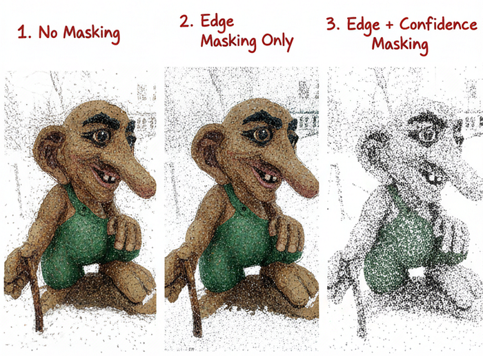
🦚 Florent's Note: I recommend starting with the defaults shown here (masking enabled, confidence disabled). Run inference. Visualize results. If you see edge artifacts, they're gone. If the reconstruction seems too sparse, you're fine. Only enable confidence masking if you observe ambiguous regions in the output — typically happens with textureless surfaces like white walls or glass.

From there, we will tweak the inference to return a list of prediction dictionaries. One dictionary per input view.

Step 6: Extracting per view 2D / 3Delements

Each dictionary should contain eleven keys—three categories: geometry outputs, camera outputs, and quality metrics:

for i, pred in enumerate(predictions):
    
    # Geometry outputs
    pts3d = pred["pts3d"]                     # 3D points in world coordinates (B, H, W, 3)
    pts3d_cam = pred["pts3d_cam"]             # 3D points in camera coordinates (B, H, W, 3)
    depth_z = pred["depth_z"]                 # Z-depth in camera frame (B, H, W, 1)
    depth_along_ray = pred["depth_along_ray"] # Depth along ray in camera frame (B, H, W, 1)

    # Camera outputs
    ray_directions = pred["ray_directions"]   # Ray directions in camera frame (B, H, W, 3)
    intrinsics = pred["intrinsics"]           # Recovered pinhole camera intrinsics (B, 3, 3)
    camera_poses = pred["camera_poses"]       # OpenCV (+X - Right, +Y - Down, +Z - Forward) cam2world poses in world frame (B, 4, 4)
    cam_trans = pred["cam_trans"]             # OpenCV (+X - Right, +Y - Down, +Z - Forward) cam2world translation in world frame (B, 3)
    cam_quats = pred["cam_quats"]             # OpenCV (+X - Right, +Y - Down, +Z - Forward) cam2world quaternion in world frame (B, 4)

    # Quality and masking
    confidence = pred["conf"]                 # Per-pixel confidence scores (B, H, W)
    mask = pred["mask"]                       # Combined validity mask (B, H, W, 1)
    non_ambiguous_mask = pred["non_ambiguous_mask"]                # Non-ambiguous regions (B, H, W)
    non_ambiguous_mask_logits = pred["non_ambiguous_mask_logits"]  # Mask logits (B, H, W)

    # Scaling
    metric_scaling_factor = pred["metric_scaling_factor"]  # Applied metric scaling (B,)

    # Original input
    img_no_norm = pred["img_no_norm"]         # Denormalized input images for visualization (B, H, W, 3)

Geometry outputs:

• pts3d: 3D coordinates in world frame (meters)
• pts3d_cam: 3D coordinates in camera frame
• depth_z: Z-depth (perpendicular to image plane)
• depth_along_ray: Depth along viewing ray

Camera outputs:

• intrinsics: 3x3 camera calibration matrix
• camera_poses: 4x4 cam-to-world transformation
• cam_trans: Translation vector
• cam_quats: Rotation as quaternion
• ray_directions: Per-pixel ray directions

Quality metrics:

• conf: Per-pixel confidence scores
• mask: Combined validity mask (edges + ambiguity)
• non_ambiguous_mask: Regions with clear geometry
• Additional: img_no_norm (original RGB), metric_scaling_factor (scale normalization)

You'll primarily use three: pts3d (world coordinates), mask (validity), and img_no_norm (colors).

🌱 Growing Note: The complete output enables advanced workflows. Use intrinsics and camera_poses to render novel views. Use depth_z for normal estimation. Use conf for uncertainty visualization. We're ignoring most of these for basic reconstruction, but production systems leverage them extensively.

When the inference finished and the predictions are stored we still have PyTorch tensors on GPU. How do we actually see the geometry?

Step 6: Decoding Prediction Tensors and Understanding Data Types

Predictions exist as CUDA tensors.

You can't directly visualize them. You can't save them to files. You can't manipulate them with standard tools (at least not directly).

Conversion to NumPy is a necessary stage. So let us loop over each element to gather the necessary outputs

#%% Step 5. Understanding and Converting Data Types
np_pts3d = np.asarray(pts3d.cpu())

pcd = o3d.geometry.PointCloud()
pcd.points = o3d.utility.Vector3dVector(np_pts3d[0][1])
o3d.visualization.draw_geometries([pcd])

The .cpu() method moves tensors from VRAM to RAM. Then np.asarray() creates NumPy views without copying data.

Before building the full pipeline, verify basic geometry:

# Create simple Open3D point cloud from first view
pcd = o3d.geometry.PointCloud()
pcd.points = o3d.utility.Vector3dVector(np_pts3d[0][1])
o3d.visualization.draw_geometries([pcd])

This should display a partial reconstruction. It won't look complete — it's only one line from one view.

🦥 Geeky Note: The world coordinate system MapAnything uses is arbitrary but consistent across views. The first image typically defines the origin. Subsequent images transform relative to this anchor. This is why single-view visualization shows reasonable structure — the model predicts metrically-scaled coordinates, not normalized depths.

Now, let see a complete single biew reconstruction

Step 7: Extracting Valid 3D Points with Mask Filtering

Not every pixel prediction is valid.

Transformers hallucinate at image edges. They struggle with occlusions. They generate ambiguous geometry for textureless regions.

The mask filters these problematic predictions. The function handles dimensionality variations. Some predictions have a batch dimension, others don't. The code adapts automatically:

#%% Step 7. Single View Point Extraction Function
def extract_points_from_prediction(prediction, apply_mask=True):
    """Extract valid 3D points and mask from a single view prediction."""
    pts3d = prediction["pts3d"].cpu().numpy()
    
    if pts3d.ndim == 4:
        pts3d = pts3d[0]
    
    if apply_mask and "mask" in prediction:
        mask = prediction["mask"].cpu().numpy()
        if mask.ndim == 4:
            mask = mask[0, :, :, 0]
        elif mask.ndim == 3:
            mask = mask[0]
        mask_bool = mask > 0.5
    else:
        mask_bool = np.ones((pts3d.shape[0], pts3d.shape[1]), dtype=bool)
    
    points = pts3d[mask_bool]
    return points, mask_bool

Mask values range [0.0, 1.0]. Values below 0.5 are invalid. Above 0.5 are valid. This binary split is standard for neural network masks. But why exactly 0.5?

The model outputs logits converted to probabilities. 0.5 represents equal confidence in valid vs invalid. Higher thresholds (0.7, 0.8) make filtering more aggressive. Lower thresholds (0.3) keep more points but include noise.

🦚 Florent's Note: I experimented with adaptive thresholding — computing optimal values per image based on confidence distributions. Results? Minimal improvement for 10x complexity. The 0.5 fixed threshold works remarkably well across diverse subjects. Sometimes simpler is genuinely better.

I use points = pts3d[mask_bool] for filtering. This is NumPy's boolean indexing. It selects only elements where the mask is True. Extremely efficient — operates at C speed under the hood.

The alternative — explicit loops checking each pixel — would take seconds.

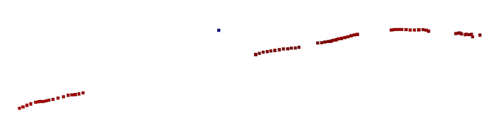
Now to visualize, you can use the following:

# Test on first view
points_view0, mask_view0 = extract_points_from_prediction(predictions[0])
print(f"View 0: Extracted {points_view0.shape[0]:,} valid points")

# Visualize single view
pcd_view0 = o3d.geometry.PointCloud()
pcd_view0.points = o3d.utility.Vector3dVector(points_view0)
pcd_view0.paint_uniform_color([0.7, 0.3, 0.3])  # Red for first view
print("Visualizing first view only...")
o3d.visualization.draw_geometries([pcd_view0], window_name="View 0 Only")

which returns:

But monochrome point clouds lack visual appeal. Where's the color?

Step 8: Mapping RGB Colors from Source Images

Each 3D point corresponds to a specific pixel.

That pixel has an RGB color in the original image. We need to map these colors to points.

The challenge: images were normalized during preprocessing. Pixel values transformed from [0, 255] to ImageNet-standardized floats.

We need the original RGB values.

Fortunately, MapAnything stores denormalized images: img_no_norm in each prediction.

So let me define the function that mirrors point extraction logic (Use the same mask indices. Access the denormalized image. Extract corresponding colors):

def extract_colors_from_prediction(prediction, mask_indices):
    """Extract RGB colors for valid points from the input image."""
    img = prediction["img_no_norm"].cpu().numpy()
    
    if img.ndim == 4:
        img = img[0]
    
    colors = img[mask_indices]
    colors = np.clip(colors, 0.0, 1.0)
    return colors

🦥 Geeky Note: The denormalization process reverses ImageNet standardization — multiplies by standard deviation, adds mean. For RGB channels, this is roughly: pixel = (normalized * 0.229) + 0.485 for red, with different constants for green/blue. The clipping handles edge cases where numerical errors push values to 1.02 or -0.01.

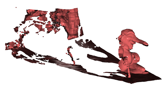
To test, you can apply colors to the first view:

colors_view0 = extract_colors_from_prediction(predictions[0], mask_view0)
pcd_view0.colors = o3d.utility.Vector3dVector(colors_view0)
print(f"Applied {colors_view0.shape[0]:,} RGB colors to view 0")

# Visualize with colors
print("Visualizing first view with colors...")
o3d.visualization.draw_geometries([pcd_view0], window_name="View 0 with Colors")

The troll should now appear in natural colors. Gray stone. Green moss:

If colors look wrong:

• Too bright/dark: Check denormalization applied correctly
• Strange hues: Color channel order might be wrong (RGB vs BGR)
• Grayscale: Colors weren't actually assigned

Now that we have a single view colored, thirty-three more views are waiting. Time to merge everything. But how do we do that?

Step 9: Merging Multi-View Predictions into Complete Reconstruction

Each view provides a partial reconstruction.

Combine all thirty-four views, and you get complete 360° coverage.

The merging process is straightforward: extract points and colors from each view, then stack vertically.

def merge_all_views_to_pointcloud(predictions, apply_mask=True, verbose=True):
    """Merge all view predictions into a single Open3D point cloud with RGB colors."""
    
    all_points = []
    all_colors = []
    
    for i, pred in enumerate(predictions):
        points, mask = extract_points_from_prediction(pred, apply_mask=apply_mask)
        colors = extract_colors_from_prediction(pred, mask)
        
        all_points.append(points)
        all_colors.append(colors)
        
        if verbose:
            print(f"View {i+1}/{len(predictions)}: {points.shape[0]:,} points")
    
    merged_points = np.vstack(all_points)
    merged_colors = np.vstack(all_colors)
    
    if verbose:
        print(f"\n✅ Total merged points: {merged_points.shape[0]:,}")
    
    pcd = o3d.geometry.PointCloud()
    pcd.points = o3d.utility.Vector3dVector(merged_points)
    pcd.colors = o3d.utility.Vector3dVector(merged_colors)
    
    return pcd

Point clouds are just lists of XYZ coordinates. Vertical stacking concatenates arrays along the first dimension—exactly what we need to merge point sets.

For thirty-four images with 30% invalid pixels masked:

• Per-view points: ~130,000
• Total merged points: ~4.5 million

This fits comfortably in 16GB RAM.

🦚 Florent's Note: First time I ran this on a medieval church dataset, seeing 50 million points accumulate felt like magic. Each individual view looked fragmented. The merged result? Complete, detailed, museum-quality. This is the power of multi-view aggregation — the whole truly exceeds the sum of parts.

Coordinate System Consistency

A critical assumption: all views share the same world coordinate system.

MapAnything ensures this during inference. The model predicts camera poses that align all views automatically. You don't manually register or align anything.

This is fundamentally different from traditional photogrammetry where you'd run bundle adjustment to refine alignment. The transformer learned to output consistent coordinates.

Occasionally, views misalign (drift over large scenes). For cultural heritage documentation at the sub-meter scale, this should be manageable. For precision engineering, we need to apply ICP post-processing.

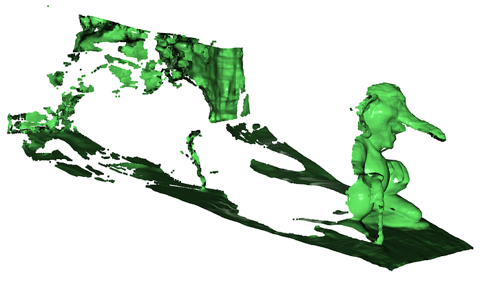
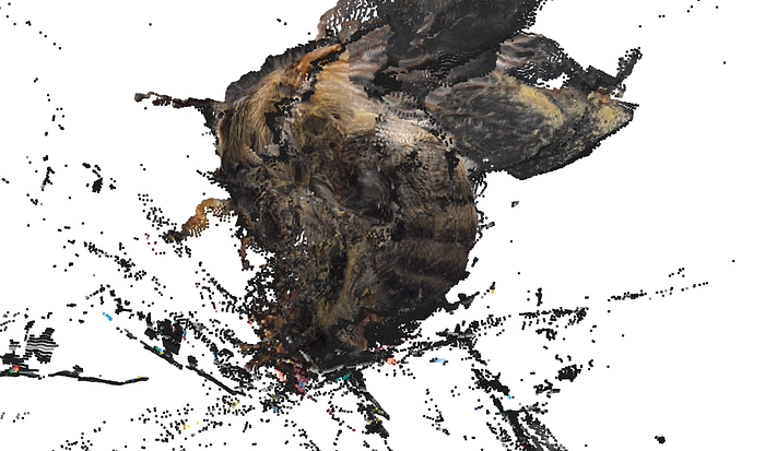
pcd_complete = merge_all_views_to_pointcloud(predictions, apply_mask=True, verbose=True)

# Visualize complete reconstruction
o3d.visualization.draw_geometries([pcd_complete], window_name="Complete 3D Reconstructions")

The visualization should show the complete troll from all angles.

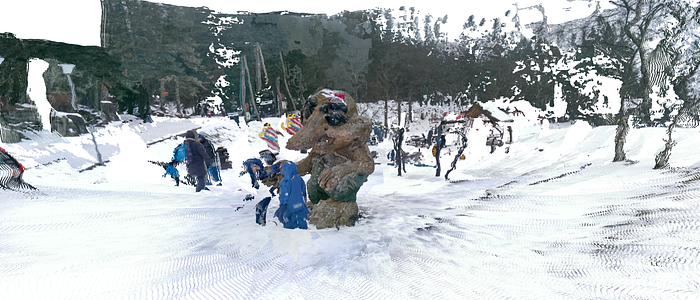
Rotate the view. Zoom in on details. The geometry should be coherent

Complete 3D model constructed. But it only exists in memory. How do we save it?

Step 10: Exporting to Standard 3D Formats

PLY (Polygon File Format) is the de facto standard for point clouds.

It's simple. It's widely supported. It stores XYZ coordinates and RGB colors efficiently. Open3D handles export in one line:

output_file = "../RESULTS/troll.ply"
o3d.io.write_point_cloud(output_file, pcd_complete)

The file writes in binary PLY format by default — compact and fast to load. For 4.5 million points with colors, expect ~110 MB file size, which you can load externally:

Alternative formats:

• XYZ: Text-based, simple, but huge files
• PCD: Point Cloud Data format (PCL library)
• LAS/LAZ: LiDAR standard, includes metadata
• OBJ/STL: Mesh formats (requires surface reconstruction first)

🌱 Growing Note: For production workflows, add metadata to exports. Open3D doesn't natively support custom metadata in PLY, but you can manually edit the header to include camera poses, capture date, or processing parameters. This makes reconstructions self-documenting.

Post-Processing Considerations

The exported point cloud is raw — direct from inference with masking applied.

Common post-processing steps:

Statistical outlier removal: Filters isolated points using KNN distance metrics. Open3D: pcd.remove_statistical_outlier(nb_neighbors=20, std_ratio=2.0)

Voxel downsampling: Reduces point density while preserving structure. Open3D: pcd.voxel_down_sample(voxel_size=0.01)

Normal estimation: Computes surface normals for rendering or meshing. Open3D: pcd.estimate_normals(search_param=o3d.geometry.KDTreeSearchParamHybrid(radius=0.1, max_nn=30))

Surface reconstruction: Generates mesh using Poisson or Ball-Pivoting. Poisson is robust: o3d.geometry.TriangleMesh.create_from_point_cloud_poisson(pcd, depth=9)

We're skipping these to focus on MapAnything's core workflow. But professional pipelines integrate them for final deliverables, and you can develop these skills + code at the 3D Geodata Academy

🦥 Geeky Note: PLY's binary format uses little-endian encoding by default. Some legacy software expects big-endian. Open3D writes little-endian, which works everywhere modern. If you encounter compatibility issues with ancient viewers, export to ASCII PLY instead (much larger files but universal compatibility).

Complete workflow executed. Thirty-four smartphone images became 4.5 million accurate 3D points with natural colors. Exported to industry-standard format. Ready for museum integration.

But where does this technology go next?

Future Directions and Advanced Applications

MapAnything represents the current state of zero-shot 3D reconstruction.

The next evolution is already emerging. Let's explore where this technology leads.

Real-Time Reconstruction on Mobile Hardware

Current limitation: MapAnything requires desktop GPUs.

The transformer is large. Inference is slow on mobile chips. But model compression is advancing rapidly.

Within two years, expect smartphone apps that reconstruct 3D in real-time as you capture. Quantization, pruning, and knowledge distillation will shrink MapAnything to 100MB models running at 30fps on Apple Silicon and Snapdragon.

This enables AR glasses that reconstruct your environment continuously. No pre-mapping. No beacons. Just immediate spatial understanding from visual input.

🪐 My Future Outlook: The killer app isn't cultural heritage or construction. It's spatial search. Imagine Googling not keywords, but 3D structures. "Find me a chair like this one" while pointing your phone. The internet becomes searchable by geometry, not just text. Foundation models make this feasible.

Integration with Large Language Models

MapAnything outputs geometry. LLMs understand semantics.

Combine them, and you get spatial intelligence. The model doesn't just reconstruct the troll — it identifies "carved troll statue, Norwegian folklore style, approximately 2.5m tall, weathered granite."

This semantic enrichment transforms raw 3D data into queryable spatial knowledge graphs. Museums could search their collections: "Show me all wooden artifacts from the 15th century with decorative carvings."

🦚 Florent's Note: To create such a solution, your best support is the Innovation Stack to make sure you can do it all: ideate, build, and ship 3D Spatial AI Innovations.

Embedding in Custom 3D Applications

MapAnything's power lies in its modularity.

Export camera poses and integrate with game engines. Export depth maps and enable portrait mode in custom cameras. Export confidence masks and drive quality control pipelines.

The framework is Apache 2.0 licensed (for the open variant). You can embed it in commercial products. Build a real estate virtual tour generator. Create a museum exhibit scanner. Develop a construction progress monitoring dashboard.

The transformer does the hard work — geometry prediction. You build the application layer.

🍉 Business Idea: Cultural heritage organizations need digital archives but lack technical expertise. Build a managed service: customers upload images via web portal, your backend runs MapAnything on cloud GPUs, they download complete 3D models with viewing software. Charge per reconstruction or subscription tiers.

Target UNESCO world heritage sites, university museums, and government cultural departments. Your moat isn't the technology (it's open source), it's the workflow integration and domain expertise.

Comparison to Traditional Photogrammetry

MapAnything trades some accuracy for enormous flexibility.

Accuracy: Professional photogrammetry achieves millimeter precision with proper GCPs (ground control points) and careful calibration. MapAnything can reach ten-centimeter-level accuracy without any calibration.

Speed: Photogrammetry requires hours of feature matching and bundle adjustment. MapAnything completes in minutes.

Ease of use: Photogrammetry demands expertise. MapAnything demands GPUs.

For cultural heritage documentation, centimeter accuracy usually suffices. You're preserving form, texture, and spatial relationships — not measuring structural tolerances.

For precision engineering or legal documentation, stick with photogrammetry. For rapid digital twins, accessible 3D capture, and AI-powered workflows, MapAnything could be useful as well.

Adding Geometric and Semantic Priors

Current MapAnything is generic — it makes no assumptions about your subject.

Future versions will integrate priors. Tell the model "this is a building" and it enforces architectural constraints (vertical walls, horizontal floors). Reconstruction quality improves dramatically with semantic guidance.

This requires fine-tuning or conditioning mechanisms. The architecture supports it. Implementation is coming.

Similarly, geometric priors like known dimensions or reference objects enable metric scaling. Right now, MapAnything's scale is consistent but arbitrary. Add a "this object is 30cm" annotation, and everything scales correctly to real-world measurements.

The Path Forward

This tutorial gave you a complete reconstruction pipeline. From smartphone photos to museum-ready 3D.

The technology will evolve. Models will compress. Accuracy will improve. Speed will increase.

But the fundamental skill — understanding transformer-based geometry prediction, configuring inference parameters, processing multi-view predictions — remains valuable.

You now have that foundation. Where you take it determines your impact.

The Bergen troll was your mission case. The framework generalizes to anything: archaeological artifacts, architectural details, industrial equipment, natural formations. The subject changes. The pipeline remains.

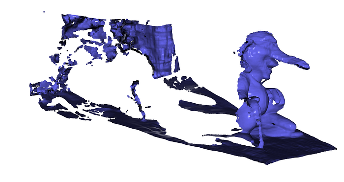
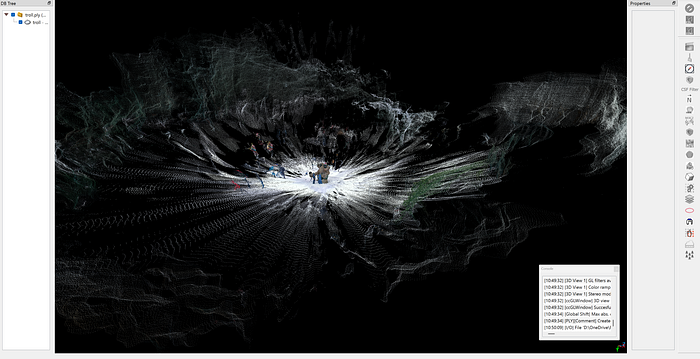
Below are some rough examples. First, I took some screenshots of a 3D Gaussian Splatting model, to see the results:

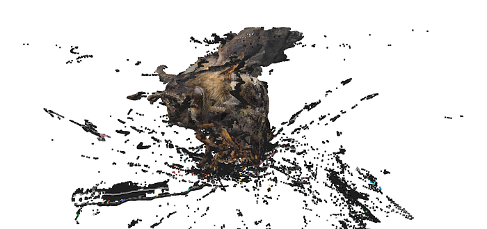
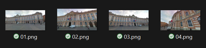
The merging is not quite there, but single-depth views are great! Then, I took some screenshots from Google Street view (4), and made it on purpose to have awful image quality:

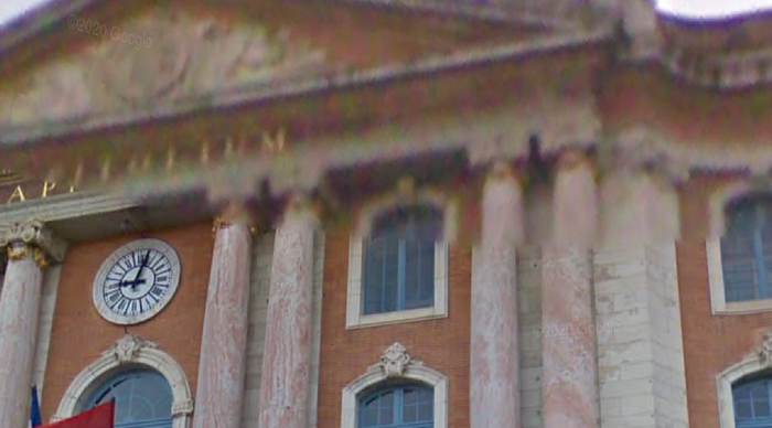
Nevertheless, here is the result (Le Capitole, in Toulouse):

This is the power of learned priors. The transformer internalized spatial reasoning from millions of examples. Your thirty-four images simply activate that knowledge for your specific subject.

Traditional photogrammetry required you to understand bundle adjustment, feature descriptors, sparse-to-dense reconstruction cascades. MapAnything requires you to understand tensor operations, parameter trade-offs, and coordinate systems.

Different skills. Same outcome. Dramatically lower barrier to entry.

You've built a persistent asset — not just a 3D model, but expertise in transformer-based spatial AI. This expertise transfers to related domains: depth estimation, novel view synthesis, 3D generation.

Warren Buffett talks about compound interest. Charlie Munger talks about mental models. This tutorial gave you both — a technical capability that improves with repetition, and a conceptual framework that extends beyond 3D reconstruction.

The cultural heritage mission from Step 2? You solved it. Thirty-four smartphone photos. One Python script. Museum-quality digital preservation.

Your Next Move

You've completed the mission. Congratulations!

Knowledge without application fades. Action cements understanding.

Here's your immediate next step: Capture something meaningful to you.

Not a test subject. Something you care about. A family heirloom. A neighborhood landmark. A local sculpture. Something where the 3D model has personal or community value.

Use the exact workflow from this tutorial. Thirty images minimum. Varied viewpoints. Consistent lighting.

Run the pipeline. Debug the inevitable issues. Adjust parameters based on your specific subject.

Share the result. Post it online. Show friends. Donate it to local archives.

This single project does three things:

1. Validates your understanding — You can't fake execution
2. Reveals gaps — Real projects expose what tutorials miss
3. Builds portfolio — Tangible evidence of capability

The second project goes faster. Parameter choices become intuitive. Error messages make sense. Results improve.

By project five, you're not following tutorials. You're solving novel problems. Adapting the workflow for specific constraints. Teaching others.

This is mastery through iteration.

Beyond personal projects, consider these directions:

Go deeper: Study transformer architectures. Read the MapAnything paper. Implement attention mechanisms from scratch. Understanding the math separates users from builders.

Go broader: Explore related techniques. Try DUSt3R for comparison. Experiment with 3D Gaussian Splatting. Learn traditional photogrammetry as contrast. Depth breeds perspective.

Go professional: Integrate MapAnything into commercial workflows. Build client deliverables. Develop specialized pipelines for specific industries. Capability becomes valuable when applied strategically.

To do all three, download an Operating System from the 3D Geodata Academy

📦 Resources

I created a special standalone episode, accessible in this Open-Access Course. You will find:

1. The complete tutorial with under-the-hood tricks📜
2. The whole dataset to download️ 📂
3. The code implementation with a permissive license💻
4. Additional resources (cheat sheet, paper …)🌍

🦚Florent: This is all offered 🎁, and based on the book below. Feel free to get it to support this knowledge sharing initiative.

Resources for Going Further

1. MapAnything GitHub Repository

The official codebase and documentation. Study the implementation details. Read the issues for common problems and solutions. Check releases for updates and improvements.

Why this resource: Source code is ground truth. Documentation tells you what should work. Code shows what actually works. The gap between them teaches you practical debugging.

2. 3D Reconstructor OS — Complete Professional Track

My comprehensive course covering the entire 3D reconstruction pipeline. From drone photogrammetry to AI-powered systems to AR/VR delivery. This tutorial introduced MapAnything specifically — the full course teaches the broader context: when to use transformers vs traditional methods, how to integrate multiple data sources, and how to build production-ready systems.

Why this resource: Context transforms technique into strategy. You need to understand not just how MapAnything works, but when to deploy it, how to combine it with other approaches, and how to deliver professional results. The course provides that strategic layer.

3. "3D Data Science with Python" — O'Reilly Book

My 687-page deep dive into spatial data processing. Chapters on point cloud analysis, 3D deep learning, and production systems. MapAnything appears in the neural 3D reconstruction section with mathematical foundations and implementation patterns.

Why this resource: Tutorials teach workflows. Books teach principles. The book explains why these architectures work, not just how to use them. Understanding foundations enables you to adapt techniques as tools evolve.

4. Open3D Documentation and Tutorials

Open3D powers your visualization and geometry processing. Their documentation covers point cloud operations, mesh generation, registration algorithms, and visualization techniques. Essential for post-processing MapAnything outputs.

Why this resource: MapAnything gets you to 3D points. Open3D takes you from points to deliverables — meshes, normals, surfaces, renderings. Mastering both tools creates complete pipelines.

Enjoyed this deep dive into transformer-based 3D reconstruction? Explore the complete 3D Reconstructor OS for professional photogrammetry workflows, AI system integration, and production deployment strategies. Or start with my book, "3D Data Science with Python", to build your spatial AI foundations from first principles.

About the author

Florent Poux, Ph.D. is a Scientific and Course Director focused on educating engineers on leveraging AI and 3D Data Science. He leads research teams and teaches 3D Computer Vision at various universities. His current aim is to ensure humans are correctly equipped with the knowledge and skills to tackle 3D challenges for impactful innovations.