
The practice of Site Reliability, more specifically, Chaos Engineering, has become more mainstream in recent times. From the engineering squads of Netflix and Google where the practice can trace its foundations, to SRE engineers in small retail websites, 'reliability' is an important measurement of success!
Running reliable services and products requires not only requires 'observable' data but also analysis and actionable insights. Observability not only helps you to avoid failures but to manage them as well.
In the practice of Chaos Engineering, observability plays a key role. Validation of hypothesis, steady state behaviour, simulating real-world events, optimizing blast radius are all those stages of your experiments where observability plays a key role.
Simply put,
Chaos Engineering — Observability = Chaos
Your systems are always generating data. Key is to clearly identify what can be used for observability and how. Well architected systems ensure robust telemetry of this data. While conducting your experiments, this data must be readily accessible.
Observability in Chaos Engineering
Observable Data in Chaos Engineering underlines following key attributes:
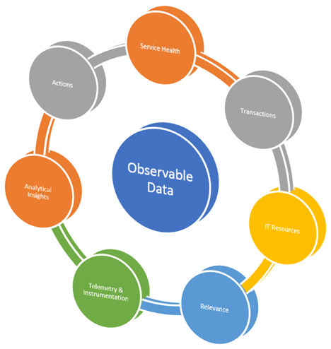
Service Health: Metrics that can tell if the service is healthy or not. Usually, a micro service exposes a URL which can respond to a GET request with HTTP 200 if certain internal checks are passed. Sometimes metrics like errors/min are also a good indicator of health and request patterns of a micro service.
Transactions: Metrics that are KPIs of business transactions that get executed through the micro service. These could be KPIs like logins/sec, checkouts/min, searches/sec or submits/hour.
IT Resources: Metrics that provides insights into IT resource utilization by the micro service. They are typically CPU Utilization, Network IO, Disk read/writes, etc.
Relevance: This attribute helps identify which metric is useful for what, e.g. submits/hour can be useful for both operations and business whereas 'credit card type per week' is useful for business product owners. Observable data should be channelled to relevant stakeholders appropriately, e.g. using specific dashboards.
Telemetry & Instrumentation: These are tools used to collect, aggregate, stream, store and analyse observable data. They are the single most important component through which you can understand and observe your chaos experiments.
Analytical Insights: These are platforms that can analyse your data. They usually see patterns in observable data and provide correlation, forecasting, regression and learning capabilities.
Actions: These are the jobs that get executed when either a simple or complex action rule is triggered. These are typical responses to events produced as part of observable data in your micro service, e.g. add 2 more containers when peak load exceeds 100 searches/sec or restart a JVM when more than 25 long running threads are detected and CPU utilization is above 90% for last 10 minutes.
When designing your experiments, it is important to understand the role each of these attributes play. For example, your experiment to test the behaviour of searches/sec transaction might get affected if you do not have access to at least service health, transaction and IT resource utilization data. If you do not have dashboards that show operations and business metrics separately, your ability to observe the steady state of your micro services is hampered. Without proper instrumentation tools you cannot provide developers the insights they require to fix the identified broken code. Without proper Analytical Insights you cannot confidently say that increase in 'submits/hour' load affects which backend network traffic bandwidth and by how much or vice versa.
In Chaos Engineering, these 7 attributes reflect not only the maturity of your experiments but the also the maturity of your 'observability' into your micro services. As you expand the practice of SRE into your teams, these attributes prominently start defining the Observability of your business.
Sources of Observable Data
We will highlight these seven attributes in action by conducting a chaos experiment. The fundamental pillars of observability are logs, metrics and traces. They provide us the data on which an observation can be made. The four golden signals in a service mesh, viz. latency, traffic, errors & saturation provide us the fundamental data set used for observations. One can find these signals embedded in logs, in your application or infrastructure metrics and even in end-to-end traces.
Traffic can be observed across all three pillars for observability. Commonly available data for traffic comes from web logs like access logs, proxy logs, load metrics from APM, request event streams or mining your application traces.
Latency is observable by measuring the time difference between request and response and analyzing the distribution of that across various actors like client, server, network, communication protocols, etc. Latency can also be measured across all pillars of observability. One can calculate latency using client side or server side monitoring agents, through trace and web logs.
Errors as opposed to their name are an extremely valuable source of information. They provide insights into configuration issues, your application code and broken dependencies.
Saturation provides insights into the utilization and capacity of your resources. Observing the saturation of your resources gives indicators on how the system is behaving in stead-state. If you can understand the limits of your infrastructure, you can even predict it for future.
Logging is a very granular way of observing the data. It varies with how the system is behaving at a particular time. One generally needs to use this data in sophisticated ingestion and analytical engines to put context around the data.
Metrics complement logging but are easy to store as their storage requirements to do not change with changes in system behavior. They are numbers and can easily be visualized. The context can be put around metrics by using analytical methods of anomaly detection, machine learning and regression techniques.
Traces provide a deep understanding of how data flows in your system. It provides context by giving you the ability to understand local and distributed application dependency maps.
We highlight these important pillars and signals by conducting a chaos experiment on a distributed system.
Observability in Action in a Chaos Experiment
- Platform: AWS
- Target: Microservice deployed in ECS Cluster
- Observability: AppDynamics APM
- Chaos Tool: Gremlin
- Load Generator: HP Performance Center
- Attack Type: Network Packet Loss (Egress Traffic)
- Blast Radius: 100% (3 out of 3 containers)
- Duration: 29 Minutes
Application Architecture
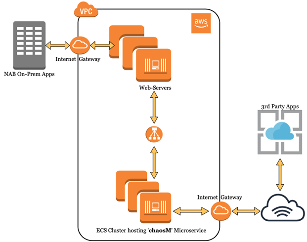
Every dependency in a distributed application is its de-facto Chaos Injection Point. Typical dependencies include compute resources, network routes, Database, 3rd-party APIs and remote services.
In this article, we specifically demonstrate a scenario of incremental network packet loss for a microservice known as 'chaosM' running as part of an AWS ECS cluster (refer diagram). The microservice is running behind a fleet of web-servers. It has 3 task definitions (ECS), balanced across 3 AWS AZs. From a functional view, 'chaosM' receives business requests from NAB's On-Prem Apps, applies the necessary transformation logic before delivering the transformed output to a 3rd-party system, residing outside NAB network. It's a backend type microservice.
Observed metrics in Steady-state and their deviations in Experiment-state help us validate the hypothesized behaviour of the concerned service.
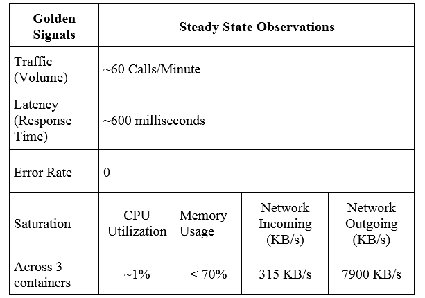
Steady State
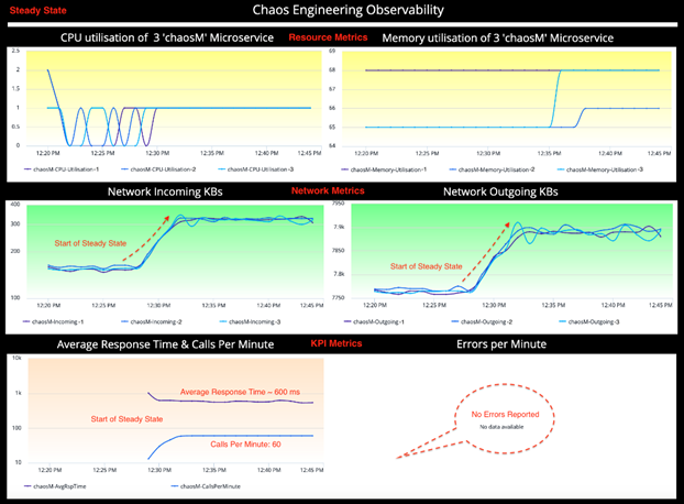
To observe the steady-state of our micro service, we use metrics called KPIs: Traffic, Errors, Latency & Saturation (Four golden signals). Depending on type of service and experiment hypothesis, the KPIs may change.
For example, our sample 'chaosM' micro service is a business integration service designed for data transformation & enrichment. Unlike customer facing services, it does not have business metrics like logins/sec, submission/minute, etc.
We have summarized the observable data into an information table. A sound understanding of the steady-state helps create a good hypothesis, one of the mandatory parameters of a Chaos Engineering experiment.
Observations:
The following information has been observed in Steady State.
Hypothesis
Based on the service's observability, we make a couple of hypothesis about the microservice:
- The incremental Packet Loss attacks of 40%, 60% & 80%, which tries to simulate varying degree of network reliability, will result in a steady increase in latency along with its corresponding error rates (HTTP 500 in this case).
- At 100% Packet Loss (a.k.a Blackhole), which simulates a downstream outage, we should be able to validate a 5 sec TCP connect timeout as configured in the 'chaosM' microservice
Design the Attack

Gremlin's Failure-as-a-Service (FaaS) Platform is used to design & launch the scenario where we execute 4 incremental network packet loss attacks with increasing intensity i.e. 40%, 60%, 80% & 100% packet loss (refer screenshot).
Each attack lasts 3 minutes. Also, a 3-minute delay is kept between each successive attack to isolate the observations and allow the service to fall back to steady state between each attack.
Therefore, the total attack window is (3 mins duration x 4 attacks) + (3 mins delay x 3) = (12 + 9) = 21 minutes.
In our observations, we also take into consideration 4 mins before & after the experiment. Hence, total observation window is 29 minutes.
Experiment State
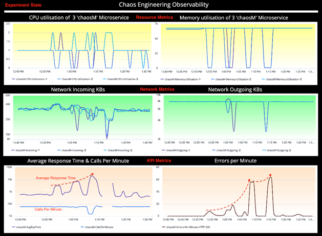
The experiment state dashboard represents the same KPIs which helps understand the behaviour of the 'chaosM' micro service when it is under attack. We will perform a comparative analysis between steady-state and experiment-state to validate the hypothesis.
A quick glance at the KPIs tells a lot about the chaos behind the scene.
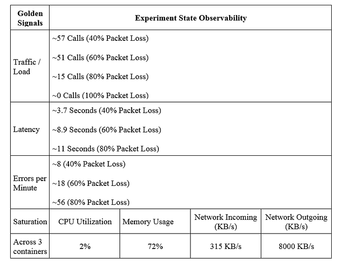
Observations:
The following information has been captured from the Chaos Engineering Dashboard in Experiment (Chaos) State.
Comparative Analysis
The technical insights generated out of the comparative analysis objectively identifies potential weaknesses (in design, coding & configurations) in the system with respect to specific categories of failures. To put things into perspective, Chaos Engineering experiments do not necessarily make your service totally immune to outages. On the contrary, among many other things, they help you uncover the known-unknowns to validate the robustness of your services.
Latency & Traffic
For the ease of comparison, we have put the SLIs from Steady and Experiment States side-by-side. While the validation of hypothesis is an important milestone, but definitely not the end goal of this experiment. There is a fair bit of explanation left to understand the behaviour of the micro service and its other associated metrics.

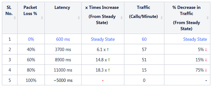
(1) While Latency of the 'chaosM' micro service is ~600 ms under the steady-state, the same shows a steady increase to 3700 ms (40% Packet Loss) and 8900 ms (60% Packet Loss) before maxing out at 11000 ms (80% Packet Loss). This rise in Latency is proportional to the magnitude of the Packet Loss attacks, which validates our first hypothesis.
(2) At 100% packet loss (Blackhole), the service has achieved the downstream outage resulting in a TCP Connection timeout at a delay of ~5 seconds based on the defined configuration. This validates our second hypothesis.
Note: The disjoint metric graph represents the Blackhole as highlighted in the above diagram.
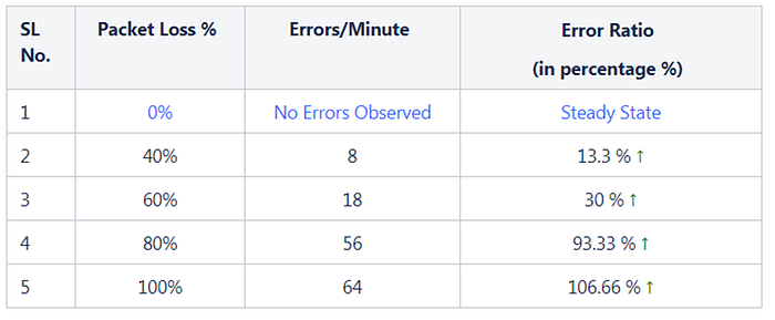
Errors
There are no Errors reported by service 'chaosM' in Steady State.
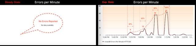
Unlike Latency, which has increased proportionally with respect to packet loss attacks, the Errors per minute metric has increased exponentially from 0 Error in Steady State to 8 Errors at 40% Packet Loss, 18 Errors at 60% and 56 Errors at 80% Packet Loss (refer screenshot). Although, it may sound a bit counter-intuitive, but these numbers proved that Chaos attacks and its effect on a micro service does not always represents a linear relationship.
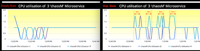
Saturation: CPU, Memory
In Steady state, the CPU utilization metric was reporting 1% across all 3 containers. The same metric in Experiment state has gone up to 2% irrespective of the magnitude of Packet loss.
The same observation holds true for Memory utilization as well. Experiment has hardly made any difference to memory utilization w.r.t. steady-state.
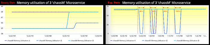
In both CPU and Memory observations, if you inspect the experiment-state graph carefully, there is a visible drop and increase in the metrics for one or more containers in every attack window marked within the dotted lines. This behavior is due to the nature of how Gremlin agents work and AppDynamics agents report the metrics in a containers (docker) environment.
In short, when one launches an attack on a docker, Gremlin by design, spins up an exact replica of the original in the same Control Group Namespace. Since, both containers now are running in the same Control Group Namespace, they share the same Process ID, IPC & network resources as shown in the diagram. Gremlin attacks the new replica container while the original one remains unaffected.
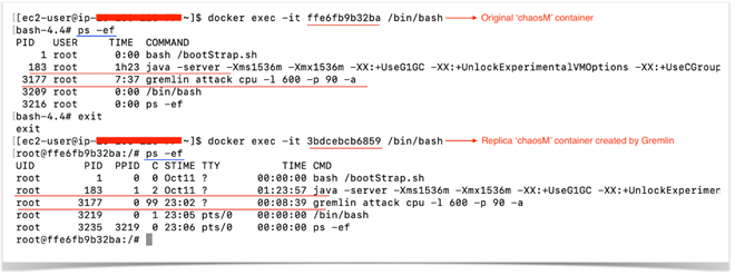
The replica container exists only for the lifetime of the attack post which Gremlin agent removes the same while the original one continues to run. Also, as the process space is also same for these two containers, the AppDynamics agent sometimes tries to report the metric from the replica container instead of the original container. It has no way to distinguish between these two. This behavior explains the anomaly observed in the CPU and Memory utilization graphs.
Saturation: Network
As highlighted in the graph, the jump in network volume is the steady-state of the micro service 'chaosM'. This metric graph is also a good indicator of the distribution of network incoming/outgoing traffic across all 3 containers deployed in each Availability Zone.
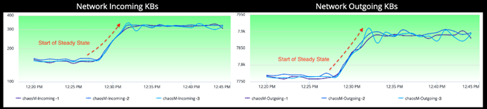
The network incoming metric in the Experiment state shows a lot of fluctuations as captured in the screenshot. If you ignore the ambient noise in the metric graph, especially at 60% & 80% Packet Loss, it shows a downward trend indicating a drop of incoming traffic while the experiment is in progress.

Since we are dropping egress network packets incrementally, i.e. 40%, 60%, 80% & 100% — the corresponding responses from the external services as well as responses back by the micro service itself are also reduced proportionally. This explains the decrease in the network incoming SLI. While the incoming metric shows 300~400 KB/s of incoming data, the corresponding network outgoing metric shows 8000 KB/s during the same time window. Due to these observations, we also concluded that unreliable network, in this case, does not affect resource utilization of our container infrastructure.
Observability for a Developer
So far, our attention has been focused on the KPIs (Latency, Traffic, Errors & Saturation) which determines the overall health of our target micro service. If the performance of the service degrades or the service fails, it would inevitably reflect in one or more KPIs. However, these metrics sometimes show the symptoms of the issue and not necessarily its underlying cause. Hence, at times we may need to look at the observability data from a different perspective.
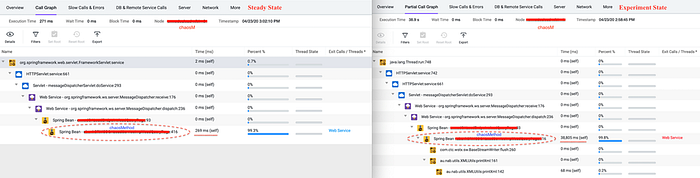
An APM monitoring solution can give us insights about the target micro service at the code level & exposes the vulnerable code segments, if any, from a Developer's perspective.
For example, the diagram above shows the waterfall model of our micro service 'chaosM' both in Steady State as well as in Experiment State. Each stage of the Waterfall model represents a segment of a code along with its execution time. The code segment Spring Bean — chaosMethod:416 took 38,805 ms or 38.8 Seconds in Experiment State which represents 99.8% of the total execution time. Whereas the same code segment only took 269 ms in Steady State. The 38.8 seconds represents the impact of the packet loss attacks on the code segment Spring Bean — chaosMethod:416.
This code level insights along with the system level visibility coming out of a monitoring (AppDynamics) helps us understand the internal workings of a micro service under various stress conditions & failure scenarios simulated through Chaos Engineering experiments. There is no place for 'guess' or 'hope' when it comes to measuring the stability of a service. The data generated out of a chaos experiment now empowers SREs & Service Owners to objectively assess the Reliability of a target service based on real world events.
To conclude
We have now seen an experiment in action. We have also seen what we call observable data. We have also given you insights into important data within observable data sets called the Golden Signals.
Observability is only of value when you better understand the data. When you look inside and answer the 'whys'. You can find answers for both Operators and Developers. You can discover the known-unknowns and unknown-unknowns once you conduct experiments on your hypothesis. Traditional resiliency testing can take you far, but only by conducting chaos experiments and investigating the observable data can you go the furthest.
This is what observability is based upon. About knowing what data to look for, what data you discover as part of experiments and building a solid understanding on your service's reliability. It's about taking that one extra step from just monitoring. Chaos experiments will not be useful if you don't understand your data the way it should be.
There is no such thing as 100% reliability but chaos experiments and the observability in those experiments help you understand why it is so and improve your customer's confidence in your services. Not just react, but observe and react well before your customers do!
If you're interested in working in technology at NAB, you can find out more here.
About the authors: Subhra Mondal is a Chaos Engineering Evangelist at NAB. He loves to learn & contribute in building NAB's Reliability Engineering Platform through adoption of Chaos Engineering.
Prateek Sachan is a Performance Management consultant at NAB. He loves everything that is about performance & reliability. He is helping NAB build its Reliability Engineering Platform.
References
- https://principlesofchaos.org/
- Cloud-native observability: https://cloud.ibm.com/docs/cloud-native?topic=cloud-native-observability-cn
- Chaos Engineering & Observability: https://www.humio.com/chaos-observability
- Pillars of Observability: https://www.humio.com/whats-new/blog/observability-redefined
- Four Golden Signals: https://landing.google.com/sre/sre-book/chapters/monitoring-distributed-systems/