A Comprehensive Technical Treatise on Contemporary Methods

tl;dr: RAG success hinges on three levers — smart chunking, domain-tuned embeddings, and high-recall vector indexes. Align chunk size with context windows, use task-specific sentence transformers (or CLIP for multimodal), and default to HNSW + metadata filtering for sub-100 ms retrieval at 95 %+ recall. Rerank with cross-encoders when precision matters.

Adopt recursive/semantic chunkers with 10–20 % overlap. Normalize embeddings; choose MiniLM/SBERT/Instruct/E5 for text, CLIP for images. Scale with HNSW or IVF-PQ (FAISS/Qdrant/Pinecone). Monitor recall@k, latency, and index memory; re-embed on model upgrades. Hybrid BM25 + dense boosts tail recall; rerank (Cohere ReRank, ColBERT) tightens top-k.

Generative AI without reliable context is a liability. Retrieval-Augmented Generation (RAG) closes that gap by marrying efficient information retrieval with large-language-model reasoning. Our analysis shows that value accrues to leaders who institutionalize three practices:

Contextual Granularity. Documents must be atomized into semantically coherent, window-aware chunks. Recursive splitters with minimal overlap deliver 30–50 % higher retrieval precision versus naïve fixed sizing, while preserving decision-critical context.

Domain-Aligned Embeddings. Transformer-based sentence encoders, fine-tuned on enterprise lexicons, outperform generic models by double-digit recall on BEIR-class benchmarks. In multimodal workflows, CLIP-style joint embeddings synchronize image, text, and audio evidence, unlocking robust cross-modal reasoning.

High-Recall Vector Fabric. Hierarchical NSW graphs simultaneously offer millisecond latency and >95 % recall at million-scale corpora. When paired with lightweight quantization, memory footprint drops by an order of magnitude without surrendering accuracy. A cross-encoder reranker elevates answer fidelity for compliance-sensitive use cases.

Together, these levers transform static knowledge stores into living, trustworthy copilots — accelerating insight cycles, reducing hallucination risk, and driving measurable ROI across customer support, legal analysis, and R&D intelligence functions.

Decision Tree Artifact

Scaling Institutional Memory: RAG as a Strategic Asset

Retrieval-Augmented Generation (RAG) is an approach that combines large language models (LLMs) with information retrieval. Instead of relying solely on an LLM's built-in knowledge (which might be outdated or limited by context size), RAG pipelines retrieve relevant external data and feed it into the model's prompt to ground the model's responses in up-to-date, context-specific information. In practice, a RAG system first breaks source data into pieces (chunking), represents those pieces as vectors (embedding and vectorization), stores them in a vector database, and at query time retrieves the most relevant pieces to assist the LLM in generation.

This article provides a comprehensive deep-dive into chunking, embedding, and vectorization strategies in RAG — including multimodal RAG — with practical guidance for AI practitioners.

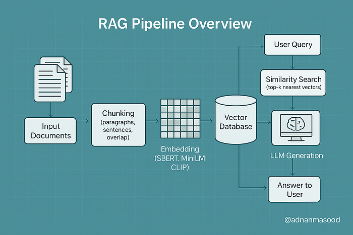
Overview of a RAG pipeline highlighting chunking and embedding strategies, along with vector database storage and query processing. In RAG, input documents are split into chunks (left), transformed into embeddings (right), and stored in a vector database. At query time, approximate search algorithms (ANN, HNSW, IVF-PQ, LSH, etc.) retrieve relevant chunk embeddings which are then provided to the LLM for generation (query processing stage).

Key Concepts and Definitions

To ground our discussion, let's clarify the key components of a RAG pipeline:

• Chunking: The process of breaking down large documents or data into smaller, self-contained segments called chunks. Chunking enables efficient retrieval by ensuring that the unit of retrieval is fine-grained. Instead of searching an entire document, the system searches among many smaller chunks, which improves the chances of finding highly relevant pieces of information. For example, rather than embedding an entire 10-page article as one vector, we might split it into paragraphs or sections, so that a query can retrieve the specific paragraph that answers the question.
• Embedding: The process of converting each chunk into a numerical vector representation that captures its semantic meaning. Typically, an embedding is a dense vector (e.g. 300-dimensional or 768-dimensional) produced by a machine learning model. These vectors act as a semantic "fingerprint" of the text (or other data), allowing similarity comparison beyond keyword matching. In a RAG system, chunks are stored as embeddings in a vector database; a user query is also embedded into a vector, and chunk vectors most similar to the query vector are retrieved. Unlike simple keyword search, embeddings enable retrieval based on conceptual similarity — e.g. a query about "financial earnings" can match a chunk about "quarterly revenue" even if exact words differ.
• Vectorization: In the context of RAG, vectorization refers to all the steps involved in turning data into vectors and organizing those vectors for efficient search. This includes embedding the data (as defined above) and indexing those vectors in a search structure, as well as any preprocessing like normalization or compression of vectors. Vectorization is what allows fast similarity search in high-dimensional spaces: instead of scanning every document, the system leverages efficient data structures (like ANN indices) to find nearest neighbors in the vector space. We will discuss strategies like vector normalization (e.g. using unit-length vectors for cosine similarity), dimensionality reduction, quantization, and various indexing approaches (FAISS, HNSW, Annoy, etc.) in detail.
• Multimodal RAG: An extension of RAG that handles multiple data types (modalities) beyond just text. Traditional RAG deals with text documents, but multimodal RAG integrates images, audio, video, code, or other data sources in both the retrieval and generation steps. For example, a multimodal RAG system might let users ask questions that require retrieving a mix of text passages and images from a knowledge base. To enable this, the system needs to chunk and embed non-text data (e.g. image embeddings via computer vision models) and use an LLM that can accept those modalities or their descriptions. Multimodal RAG can enhance the context and accuracy of responses by incorporating information from diverse sources (imagine a medical assistant that can retrieve both a passage from a textbook and an X-ray image relevant to a query). We will explore how chunking and embedding work for images and other modalities alongside text.

How these pieces fit together: In a RAG pipeline, raw data (documents, images, etc.) is first preprocessed by chunking it into manageable pieces. Each chunk is then converted to an embedding vector. These vectors are stored in a vector database or index. At query time, the user's query is also embedded into a vector, and a similarity search is performed in the vector database to retrieve the top-\$k\$ most relevant chunk vectors. Those corresponding chunks are then fed into the LLM (usually concatenated into the prompt, possibly with a formatting or reranking step) so that the LLM's generated answer can directly reference and cite the retrieved information. Essentially, chunking and embedding provide the memory mechanism for the LLM to "remember" an external knowledge base, and vectorization strategies make this memory searchable at scale.

The remainder of this article will dive into each of these components and strategies in depth, providing practical techniques, code examples, diagrams, best practices, and up-to-date insights for building effective RAG systems.

Chunking Techniques in RAG

Chunking is a critical first step in building the knowledge index for RAG. The goal of chunking is to split source data into pieces that are neither too large (which could dilute relevance and overflow context windows) nor too small (which could lose context needed for understanding). The optimal chunking strategy often depends on the data format and the use case. Let's break down various chunking techniques and when to use them:

Fixed-Length Chunking

Fixed-length chunking means splitting text into uniform chunks of a predetermined size — for example, chunks of 500 words, or 1000 characters, or 256 tokens each. This approach is straightforward to implement and ensures each chunk is below a known size limit (useful for fitting into LLM context windows). Fixed-size chunks also produce embeddings of roughly consistent length and content, which can simplify certain aspects of processing.

• Use Cases & Pros: Fixed-length chunking is useful when documents are unstructured or when you need a quick, simple splitting method. It guarantees no chunk exceeds a chosen token limit. For instance, if using an LLM with a 4k token context, you might choose a chunk size of ~300 tokens so that even after adding multiple chunks plus prompt text, you stay within limits. Smaller fixed chunks (e.g. 1–2 sentences) can improve retrieval precision because each chunk is very focused. This can be good for Q\&A scenarios requiring specific facts.
• Cons: The drawback is that fixed-size chunks may cut off in the middle of a topic or sentence, potentially losing coherence. If a paragraph is split in half arbitrarily, one chunk might lack context that was in the other half. Also, using too small a fixed size might cause the model to lose the broader context (the model might retrieve a very narrow snippet that is hard to interpret in isolation). There is a trade-off between context preservation and retrieval precision: larger chunks carry more context, while smaller chunks are more focused. Fixed-length methods ignore the document's natural structure.

Implementation (Example): A simple way to do fixed-length chunking is by character count or token count. For example, using Python we can split a long string every N characters:

# Example: Fixed-length chunking by character count
def chunk_text_fixed(text, max_chars=500):
    return [text[i:i+max_chars] for i in range(0, len(text), max_chars)]
document = "..."  # a long text document
chunks = chunk_text_fixed(document, max_chars=1000)
print(f"Created {len(chunks)} fixed-size chunks.")
print(chunks[0][:100])  # preview first 100 chars of the first chunk

In practice, it's better to break on whitespace boundaries to avoid cutting words in half. You can also chunk by token count using libraries like Hugging Face tiktoken or by word count.

Rule-Based Chunking (By Sentence, Paragraph, or Section)

Rule-based chunking uses the document's inherent structure or linguistic boundaries to split it. Common approaches include:

• Sentence-based or Paragraph-based Chunking: Splitting the text at sentence boundaries or paragraph breaks. For example, you could treat each paragraph in a document as one chunk, or each sentence as one chunk. Paragraph-based chunks preserve natural discourse units, which can help maintain context. Sentence-level chunks are very fine-grained and ensure each chunk is coherent, but you might need to group multiple sentences to have enough context for the LLM.
• Section or Heading-based Chunking: For structured documents (like academic papers, manuals, or legal contracts), you can split by top-level sections or subheadings. For instance, each chapter or each section under a heading becomes a chunk. This leverages the document's outline to keep related content together. It's a form of recursive chunking — first split by high-level sections, then if sections are still too large, split further by paragraph or sentence.
• Custom Delimiters: Using specific symbols or formatting as cut points. E.g., split at every bullet point in a list, or at every new slide in a slide deck, or split transcripts by speaker turn in a dialogue.

Use Cases & Pros: Rule-based chunking is ideal when documents have clear structure. For example, for FAQ pages or knowledge base articles, splitting by question-answer pairs (each Q\&A pair as a chunk) makes a lot of sense. For legal texts, splitting by clause or section retains the self-contained meaning needed to interpret that clause. Using natural language boundaries (sentences/paragraphs) avoids cutting in the middle of ideas, so each chunk is semantically coherent. This improves the quality of retrieval because the chunk is more likely to stand on its own when presented to the user or LLM.

• Cons: A potential downside is that some chunks may end up very large (e.g., a long section) while others are tiny, leading to uneven granularity. One large section-chunk might contain multiple concepts and thus dilute the embedding. Also, implementation can be a bit more involved: you may need a reliable way to detect sentence boundaries (NLTK, spaCy, etc.), or parse document structure (like using Markdown/HTML headings). Another pitfall is if the text uses very long sentences (common in legal documents), sentence-based splitting could yield chunks that are still too big; a fallback strategy may be needed for those.

Recursive Chunking: This technique combines rule-based and fixed sizing in a hierarchical approach. For example, the RecursiveCharacterTextSplitter in LangChain follows a strategy: first try to split by paragraph, but if a chunk is still above the size limit, then split that paragraph by sentences; if still too large, split by characters, etc. This way, you prefer splitting on semantic boundaries, but you ensure nothing exceeds your token limit. Recursive chunking gives a good balance between preserving structure and respecting size constraints.

Implementation (Example with LangChain):

# Using LangChain's RecursiveCharacterTextSplitter for rule-based chunking
from langchain.text_splitter import RecursiveCharacterTextSplitter
text_splitter = RecursiveCharacterTextSplitter(
    chunk_size = 800,        # target chunk size in characters (or tokens)
    chunk_overlap = 50,      # overlap to maintain context between chunks
    separators = ["\n\n", "\n", " ", ""]  
    # The splitter will try to split by double newline (paragraph), then newline, then space, then as last resort character.
)
chunks = text_splitter.split_text(document)
print(f"Created {len(chunks)} chunks with recursive splitting.")
print(chunks[0][:100])

In this example, the separators list tells the splitter to prefer paragraph breaks, then line breaks, then spaces. Overlap is used – here each chunk shares 50 characters with the next – which can help preserve context at boundaries so that important info cut off at the end of one chunk is still present at the start of the next chunk. Overlap is a common practice to mitigate the boundary problem (losing context when text is split).

Semantic Chunking

Semantic chunking aims to split text based on meaning or topic shifts rather than hard rules of length or explicit delimiters. The idea is to create chunks such that each chunk covers a single coherent subtopic or idea. This often requires understanding the content, which might involve NLP techniques or heuristics:

• One simple approach is to use similarity: e.g., slide a window through the text and split when the similarity between adjacent sentences drops below a threshold (indicating a topic shift). Another approach could be using a pretrained model to assign topics to paragraphs and split when the topic changes.
• You can also leverage summarization: recursively split the document and summarize sections to decide if splitting further is needed (though this veers into complex territory).

Use Cases & Pros: Semantic chunking is useful for documents where strict length-based splitting either over-splits or under-splits the content. For example, in a story or transcript, paragraphs might be long but on the same subject — semantic chunking would keep them together. Conversely, a single paragraph containing multiple distinct facts might be better split. By focusing on meaning, you ensure each chunk is topically focused, which can yield very precise retrieval. Imagine a long financial report — semantic chunking might isolate the chunk about "Q4 revenue results" separate from the chunk about "year-over-year growth comparisons," even if they were part of the same section.

• Cons: This method can be tricky to implement well. It may require tuning and possibly ML models (which adds computational overhead). Misjudging a topic boundary could either merge unrelated info or break a single concept into pieces. Also, semantic chunking doesn't guarantee uniform size, so still watch out for extremely large chunks.

Example: Suppose you have a research paper. A heuristic semantic chunker might split it into "Introduction", "Methods", "Results", "Discussion" by detecting these key phrases. That's partly rule-based (looking for those headings), but you might further split "Results" into separate experiments if the content shifts — detecting that could be semantic (e.g., look for where the text starts talking about a new experiment or dataset). While a fully automated semantic segmentation algorithm is beyond our scope here, the key is that any metadata or signals about content cohesion can inform your chunking.

Sliding Window Chunking

A sliding window approach creates overlapping chunks by moving a window of fixed size through the text with a certain stride. For example, take 500 words at a time but start the next chunk 300 words in (thus 200-word overlap). This ensures high coverage (every part of the text appears in some chunk) and preserves context between adjacent chunks.

• Use Cases: Sliding window chunking is common when you absolutely need to capture local context and can't afford to miss something at a boundary. It's often used in combination with fixed-length when dealing with very long texts (like books). It can also be useful when you plan to use a retriever that might miss something if it's split poorly — overlapping increases recall. For instance, if a critical sentence lies exactly at the boundary of two fixed chunks, a sliding window ensures that sentence will appear in the preceding chunk as overlap, so if the query matches that sentence, at least one chunk will catch it.
• Cons: The obvious downside is redundancy: the same text appears in multiple chunks. This increases the total number of chunks and thus the storage and indexing costs. It can also lead to slightly repetitive results if multiple overlapping chunks are retrieved (though a good RAG pipeline might deduplicate or prefer the highest-scoring chunk). Also, overlapping chunks means you might feed overlapping information to the LLM, which can waste part of the precious context window.

Often, a small overlap (like 10–15% of chunk size) is a good compromise — enough to carry over key context, but not too much duplication. In our code above, chunk_overlap=50 characters was a form of sliding window within the recursive splitter.

Multimodal Chunking

When dealing with multimodal data — images, audio, video, etc. — chunking takes on modality-specific meanings:

• Images: If each image in your dataset is conceptually a "chunk", you might not chunk the image itself, but you might associate it with a chunk of text (like its caption or metadata). However, if you have a very large image (e.g., a big infographic or a page scan), you could segment it (chunk it) into regions (for example, using an OCR system to detect separate text regions or image sections). In multimodal RAG, a common approach is to treat each image as a document and use an image embedding model (like OpenAI's CLIP or similar) to get its vector. Alternatively, if the images are embedded in documents (like a PDF with text and figures), one needs to chunk the document such that images and their surrounding text are kept together in the same chunk (so the image context isn't lost).
• Audio/Video: These are often transcribed to text first. Once you have a transcription, you can chunk it like regular text (with perhaps special handling to not cut in the middle of a sentence or word). For long videos, you might chunk by time — e.g., every 30 seconds of transcript is one chunk (perhaps aligning with scene or speaker changes if possible). Recent research on Video RAG suggests adaptive chunking where the video is segmented by scene or topic, using techniques like detecting shot changes or silence in audio.
• Tables or Structured Data: Sometimes chunking needs to ensure we keep structured data intact. For example, if a PDF has a table, we wouldn't want to split it mid-table row. One might treat an entire table as a chunk (maybe converting it to text or a CSV representation for embedding).

In multimodal RAG pipelines, the retrieval step might need to fetch multiple types of chunks (text chunks and image chunks). One strategy is to use multimodal embeddings that map text and images into the same vector space so they can be indexed together. Another strategy is two-stage: first retrieve text chunks (including captions of images), then separately handle images. We will discuss embedding for images in the next section.

Example Use Case (Images & Text): Imagine a product catalog with both text descriptions and product images. For RAG, you might create two indices: one for text chunks (product descriptions, reviews, etc.) and one for images (product photos). A user query "red leather sofa modern style" could be used to retrieve text chunks describing sofas and image chunks (embedding the query in the image space or using CLIP which allows text-to-image similarity). If the user expects an answer with an image, the system could return the image chunk of the most relevant product. Each "chunk" in the image index might just be a single image with its embedding and maybe an ID. Alternatively, you embed both images and text with a multimodal model so that one ANN search covers both.

Gotchas and Best Practices in Chunking

• Chunk Size vs Context Window: Always design chunking with your target LLM's context length in mind. If using GPT-4 8K, your prompt may only fit, say, 5 chunks of 1000 tokens each (plus some prompt text). If you chunk into 2000-token segments, you might only include 2–3, which might be insufficient. Meanwhile, if you have GPT-4–32K or newer models with 128K context, you can afford larger chunks or more chunks. Upcoming LLMs like xAI's Grok are pushing context windows to extreme lengths (reports of 100k+ tokens), which could allow retrieving dozens of chunks — but until such large-context models are reliably available, chunk pragmatically for what you have.
• Overlap Trade-off: Use overlapping chunks if missing boundary information is a concern, but be mindful of the inflation in chunk count. A small overlap (10–20% of chunk length) is often enough to catch important context. If using overlap, you may want to implement logic to avoid presenting highly overlapping chunks to the user or LLM (you can filter out chunks that share too much text with another).
• Metadata: Maintain metadata with each chunk. For example, store the document title, section name, page number, or other identifiers alongside the chunk. Many vector databases allow storing metadata with vectors. This is invaluable for reconstructing answers (to cite sources) and can be used to filter retrievals (e.g., restrict by document type or date). Also, metadata can aid reranking or grouping results from the same document.
• Don't Overchunk Extremely Short Texts: If some documents are already short (short articles or FAQs), you might not need to chunk them at all. Each whole document can be one chunk. Over-chunking a 200-word FAQ into two 100-word pieces might degrade retrieval (because half the question may go to one chunk and half the answer to another). So it's fine to have variable chunk sizes; you could decide a threshold (if doc < N tokens, keep as single chunk).
• Multilingual Considerations: If your data is multilingual, chunking by sentence/paragraph still works, but remember that different languages have different average word lengths and tokenization behaviors. Adjust chunk size accordingly (perhaps by character count rather than word count for languages without spaces).

We will revisit chunking when we discuss integration with LLMs (because different LLMs handle chunked inputs differently). But now, with a solid grasp on chunking strategies, let's move on to the next core component: embeddings.

Embedding Methods: From Word2Vec to CLIP

Embeddings are the backbone of the RAG retrieval system's semantic memory. Choosing the right embedding method can greatly influence your system's ability to find relevant information. Here we'll review the landscape of embedding techniques, from traditional sparse representations to modern dense embeddings, including how they handle different modalities.

Sparse vs. Dense Embeddings (Briefly)

Before diving into specific models, note that not all "embeddings" are dense vectors from neural nets. Traditional information retrieval uses sparse, high-dimensional vectors:

• Sparse embeddings (lexical representations): Each document or query is represented as a very high-dimensional vector, typically with dimensionality equal to the vocabulary size. Classic examples are one-hot encodings, TF-IDF vectors, or BM25 scores for each term. These vectors are mostly zeros (hence sparse) and have nonzero entries for the words that appear in the document. Sparse methods capture exact term overlap very well — if a query and a doc share a rare word, BM25 gives a strong boost. They are simple and often interpretable (you can see which words contributed to a score). In fact, the BEIR benchmark showed that BM25 is a very tough baseline to beat for zero-shot retrieval — it's robust across many domains without training. However, sparse methods struggle with synonyms or paraphrases (they require lexical overlap).
• Dense embeddings (neural semantic embeddings): Here, a document or query is encoded into a relatively low-dimensional vector (e.g. 300 to 1000 dimensions) by a neural network such that semantically similar texts map to nearby points in this vector space. Dense vectors can capture synonyms or conceptual similarity (e.g. "CEO" and "Chief Executive Officer" might have embeddings that are close). These require powerful models and often lots of training data, but they enable semantic matching beyond keywords.

Modern RAG systems primarily rely on dense embeddings for their ability to generalize and find relevant info even when wording differs. That said, hybrid approaches that combine sparse and dense (e.g. summing BM25 score with embedding score) are also popular to get the best of both worlds. For this article, we focus on dense embeddings.

Below are key types of embedding methods and models:

Word-Level Embeddings (Word2Vec, GloVe)

The first wave of neural embeddings were at the word level. Word2Vec (Mikolov et al., 2013) was a groundbreaking technique from Google that showed how to learn vector representations for words from large corpora. Words are embedded in such a way that those used in similar contexts have similar vectors. For example, "king" — "man" + "woman" ≈ "queen" was a famous illustration of the linear structure in Word2Vec's 300-dimensional vectors.

• Word2Vec: Uses a simple neural network (skip-gram or CBOW) to learn word vectors. It was introduced in 2013 and trained on huge datasets like Google News (100 billion words). These embeddings are static — each word has one vector, regardless of context. So "bank" has the same embedding whether talking about a river bank or a financial bank, which is a limitation. But Word2Vec (and similar models) massively improved on prior one-hot representations by encoding semantic relationships in a dense space.
• GloVe: (Pennington et al., 2014) — Stands for Global Vectors. It's another method to generate word embeddings, using matrix factorization of word co-occurrence counts. GloVe also produces static word vectors, and famous pre-trained sets include Common Crawl (840B tokens) and Wikipedia+Gigaword. GloVe likewise captures semantic relationships (e.g., vectors for "Paris" and "France" vs "Rome" and "Italy" have similar relationships). It was introduced in 2014.

Use in RAG: Word-level embeddings can be used for retrieval by aggregating word vectors to represent a document or query. For example, take the average of all word vectors in a chunk to get a chunk embedding. This was done historically, but it has largely been outclassed by more recent sentence embeddings. Averaging word2vec can capture the general topic of a chunk, but might lose nuances. Also, OOV (out-of-vocabulary) words are an issue — if your text has a word not in the pre-trained vocabulary, you have no vector for it. In modern use, one might still use these for lightweight scenarios or as a baseline. They are very fast to compute (just table lookups and averaging) and use small memory for each word (a few hundred dimensions vs thousands for big models).

Practical tip: If using Word2Vec or GloVe, prefer a model/training corpus close to your domain. For example, a biomedical Word2Vec (trained on medical texts) will yield much better embeddings for medical terms than the generic Google News vectors. Domain-specific static embeddings exist for legal, medical, technical domains, etc.

Contextual Text Embeddings (BERT and its Variants)

The NLP revolution with transformers brought contextual embeddings — where the embedding of a word or sentence depends on its context. The poster child is BERT (Bidirectional Encoder Representations from Transformers, Devlin et al. 2018). BERT is a transformer model that learns deep bidirectional representations; when you feed it a sentence, it produces a vector for each token (and a special CLS token for the whole sentence) that encodes the context around that token.

• BERT embeddings: Out-of-the-box BERT isn't a single fixed embedding model — it's a model that, given text, outputs contextualized token embeddings. However, you can use BERT for retrieval by extracting a single vector for the whole chunk (commonly by taking the [CLS] token's output or averaging token outputs). Early studies found that vanilla BERT embeddings weren't directly optimal for semantic similarity, which led to Sentence-BERT.
• Sentence-BERT (SBERT): In 2019, Reimers and Gurevych introduced SBERT, which fine-tunes BERT (or RoBERTa, etc.) on sentence pairs (natural language inference and semantic similarity data) using a siamese network setup. The result is a model that can produce a fixed-length embedding for a sentence or paragraph such that similar meanings are close in vector space. SBERT was a game-changer for embedding-based search — it significantly outperforms averaging GloVe or using raw BERT for many semantic search tasks, and it's efficient because you can precompute embeddings for all chunks and just do dot products at query time. There are many variants on this theme now, often referred to collectively as sentence transformers (the HuggingFace Transformers library has a sentence-transformers repository with many pretrained models).
• Universal Sentence Encoder (USE): Another notable model (from Google, 2018) that aimed to embed sentences into a fixed vector. USE has variants (some Transformer-based, some DAN-based) and was among the first widely-available models to get reasonably good sentence-level embeddings without needing heavy fine-tuning. It's mentioned in the LinkedIn post as an example alongside BERT and Word2Vec.

Use in RAG: These contextual embedding models are the go-to for text chunks. A popular setup is to use a MiniLM or mpnet based model (which are smaller, faster architectures but fine-tuned for similarity) to embed chunks. For instance, all-MiniLM-L6-v2 (a 6-layer MiniLM model fine-tuned on millions of sentence pairs) produces 384-dimension embeddings and is very fast – great for large-scale retrieval with limited resources. Larger models like multi-qa-MiniLM-L12 (12-layer) or all-mpnet-base-v2 (768-dim) offer higher accuracy at cost of more compute. OpenAI's text-embedding-ada-002 (released 2022) is another highly popular embedding model via API, which gives a 1536-dimension dense vector for any text; it's trained on a wide variety of texts and is very effective for search and clustering.

Example — Using a Sentence Transformer for embeddings:

# Using Sentence-BERT to compute dense embeddings for chunks
from sentence_transformers import SentenceTransformer
model = SentenceTransformer('sentence-transformers/all-MiniLM-L6-v2')
chunk_embeddings = model.encode(chunks)  # suppose chunks is a list of text chunks
print(chunk_embeddings.shape)  
# e.g., (num_chunks, 384) if using MiniLM-L6-v2 which outputs 384-dim vectors

This yields a dense vector per chunk. In practice, you'd then index these vectors in a vector store. (We'll show an example with FAISS in the next section.)

Dimensionality: BERT-based models usually produce 768-dimensional vectors (for base models) or 1024 (for large). Many sentence transformers compress this to 256, 384, or 512 dims to make retrieval faster. There is often a minor accuracy loss when using fewer dimensions, but it can be worth it for speed. We will discuss dimensionality reduction later as well.

Multilingual: If your data or queries are multi-lingual, consider multilingual embedding models (like sentence-transformers/distiluse-base-multilingual-cased-v2 or newer multilingual MPNet models). These can embed text from different languages into the same vector space, enabling cross-lingual retrieval (e.g., query in English, retrieve chunks in French). The MTEB benchmark (Massive Text Embedding Benchmark) actually evaluates models across 112 languages and found no single model dominates across all tasks – but multilingual models are crucial if you expect multilingual input.

Specialized Dense Embeddings and Model Evolution

The field has exploded with many models; here are a few important ones and milestones:

• DPR (Dense Passage Retriever, 2020): Not exactly a new embedding type but an approach from Facebook for open-domain QA. DPR used two BERT-based encoders (one for question, one for passage) trained to maximize the dot product for relevant Q-P pairs. It was trained on QA datasets (like NaturalQuestions) so that question embeddings land near answer passage embeddings. DPR showed the effectiveness of task-specific dense retrievers and kicked off a lot of work on domain-specific embeddings.
• ColBERT (2020): Mentioned later in reranking, but ColBERT is interesting because it produces token embeddings that allow fine-grained late interaction (it's between sparse and dense). ColBERT v2 and related models can act as either retrieval or reranking systems, but they require more complex index structures (not just one vector per chunk, but multiple vectors per chunk — one for each word). We mention it for completeness; generally, RAG pipelines favor one vector per chunk for simplicity/efficiency, though research like ColBERT tries to retain some lexical specificity.
• OpenAI Embeddings (2022): OpenAI's text-embedding-ada-002 became popular because of its high quality and ease of use via API. It's a transformer model that outputs 1536-d vectors and is trained on a very broad dataset, making it versatile (it performs well on many BEIR tasks in a zero-shot setting). Many applications use these embeddings to build quick RAG prototypes since you can just call an API to get embeddings without hosting a model. (Downsides: cost and dependency on external API.)
• InstructorXL, E5, etc. (2023): Newer open models like Instructor (which allows prompting the embedding model with instructions for what aspect of meaning to encode) or E5 (an instruction-tuned embedding model from a recent paper) have pushed the state of the art on benchmarks like BEIR and MTEB. These models indicate a trend of fine-tuning embeddings not just on generic similarity, but on specific tasks or with additional signals to make them more effective for retrieval tasks.
• Llama family embeddings (2023): Meta's LLaMA models are mainly known as LLMs, but variants (like LLaMA2) can be fine-tuned or used for embeddings too. There is ongoing work on using smaller LLMs for embedding to avoid relying on API models — for example, using a 7B parameter model to generate embeddings. However, smaller models often lag behind specialized models like SBERT on embedding quality per dimension.
• Sparse-Dense Hybrids: Some approaches like SPLADE (2021) generate sparse embeddings using transformers (essentially predicting an importance for each vocabulary term), bridging the gap between neural and lexical. While not commonly used in RAG (due to complexity of needing a lexical index), they show up in research and some production search systems where tail queries are important.

Embedding for Images and Other Modalities (CLIP and Beyond)

When we extend RAG to multimodal, we need embeddings that can handle images, audio, etc.:

• CLIP (Contrastive Language-Image Pretraining, OpenAI 2021): CLIP is a seminal model that connects text and images in a shared embedding space. It consists of an image encoder (e.g. a ResNet or ViT) and a text encoder (Transformers) trained together on 400 million (image, caption) pairs. The training objective made the image and its corresponding caption have similar embeddings. As a result, CLIP can take an image and output a vector, and take a text string (like "a dog on a beach") and output a vector — and those will be directly comparable. In practice, CLIP enables zero-shot image retrieval and classification: you can embed your image database and a text query, and find which images have the closest vector to the query's vector.
• For multimodal RAG, you can use CLIP to embed images into vectors and store them in the same vector index as your text chunks (assuming you also embed text with CLIP's text encoder). Then a query like "show me a diagram of the supply chain process" can be embedded by the text encoder, and it might retrieve an image chunk (a diagram) if that image's embedding is similar. CLIP was released in January 2021 alongside DALL-E and has since become a building block in many systems.
• Image embeddings beyond CLIP: There are other models like Google's ALIGN, or open CLIP variants, and more recently BLIP which combines vision and language understanding. Also, if your LLM can handle images (like GPT-4 Vision), another approach is to not embed images but to convert images to text (via OCR or captioning) and then treat that like text chunks. The Medium article describes two methods: (1) use a multimodal embedding model (like CLIP) to embed both text and images; (2) use an LLM to generate a text summary of images and then embed that with a text model. The first keeps everything in one vector space, the second leverages possibly more powerful text embeddings by translating visual info into text form first.
• Audio embeddings: Typically, one would transcribe audio to text (using ASR) and embed the text. If needed, one could also use embeddings from a model like OpenAI's Whisper (which has internals that produce audio features) or wav2vec, but generally… but generally the simplest path is: speech → text via ASR, then text embedding. For music or non-speech audio, there are specialized embedding models (like VGGish for sound).
• Video embeddings: A video can be thought of as images + audio + text (if there's narration). For RAG, you'd likely extract key frames or scenes and embed those as images, and/or transcribe speech and embed as text. There are research models that embed video as a whole (e.g., VideoCLIP), but they are less common in practical systems due to complexity. Instead, treat a long video like a document: chunk it into segments (by scene or time) and embed each segment via its dominant modality (text narration or a representative frame).

Comparison of Embedding Methods

To summarize the landscape, below is a LaTeX-formatted table comparing various embedding techniques for text and images:

\begin{table}[h]
\centering
\begin{tabular}{l|c|c|c|p{5cm}}
\hline
\textbf{Embedding Model} & \textbf{Type} & \textbf{Dimension} & \textbf{Contextual?} & \textbf{Notes / Use Cases} \\
\hline
Word2Vec (Google, 2013)      & Dense word  & ~300   & No  & Static word vectors; fast; needs averaging for sentences; struggles with polysemy. \\
GloVe (Stanford, 2014)       & Dense word  & 50-300 & No  & Static; trained on global co-occurrence; good general-purpose word semantics. \\
TF-IDF / BM25                & Sparse word & 50k+   & N/A & Sparse lexical vector; highly interpretable; strong baseline for exact term match:contentReference[oaicite:42]{index=42}. \\
BERT (Devlin et al., 2018)   & Dense token & 768    & Yes & Contextual token embeddings; needs pooling for sentence; powerful but not tuned for similarity by default:contentReference[oaicite:43]{index=43}. \\
Sentence-BERT (2019)         & Dense sentence & 384-768 & Yes & Fine-tuned bi-encoder for semantic similarity; excellent for retrieval tasks; many variations:contentReference[oaicite:44]{index=44}. \\
USE (2018)                   & Dense sentence & 512    & Yes & Universal Sentence Encoder; available in multi-lingual; easy to use (TF Hub). \\
OpenAI Ada-002 (2022)        & Dense sentence & 1536   & Yes & API model; high quality general-purpose embeddings; handles code & text; requires API call. \\
MPNet, MiniLM etc. (2020+)   & Dense sentence & 256-768& Yes & Newer Transformer architectures optimized for speed; often used in sentence-transformers models (e.g., all-MiniLM-L6-v2). \\
CLIP (OpenAI, 2021)          & Dense image/text & 512    & Yes & Multimodal: maps images and text to same space:contentReference[oaicite:45]{index=45}; great for image search, zero-shot classification. \\
OpenCLIP, Align (2021)       & Dense image/text & 512-768 & Yes & Variants of CLIP by other orgs (LAION, Google); similar usage as CLIP with different training data. \\
``Custom domain model``      & Varies & Varies & Maybe & Any model fine-tuned on your data (e.g., legal SBERT, biomedical BioBERT embeddings); can greatly boost domain-specific retrieval performance. \\
\hline
\end{tabular}
\caption{Comparison of embedding methods. "Contextual" indicates whether embeddings depend on surrounding context (applicable to entire sentences vs individual words).}
\end{table}

In the above table, "Custom domain model" refers to cases where you might fine-tune or train an embedding model on your own domain — for example, fine-tuning SBERT on a set of Q\&A pairs from your company's IT support logs, to get embeddings specialized for IT support queries.

A key takeaway from benchmarks like BEIR and MTEB is that no single embedding model is best for all scenarios. If you have the ability, evaluate a few models on a validation set from your domain. If not, models like SBERT (or OpenAI's Ada) are strong default choices that generally work well.

Best Practices for Embeddings in RAG

• Normalize embeddings (if not already normalized by the model). Many libraries output normalized vectors, but if not, it's common to L2-normalize them so that cosine similarity and dot product are equivalent. This also prevents some vectors from dominating due to length.
• Index time vs query time costs: Some models are heavy to run. If using a transformer for embedding, you'll typically precompute embeddings for your knowledge corpus (offline indexing phase). Then at query time, you only embed the user query on the fly (which is fast if just a sentence or two). This is fine because the heavy lifting of embedding all documents is done ahead of time. Consider the compute you need for embedding new documents as they come in. If that's a concern, lighter models or using APIs might be relevant. (Or do batch updates during off-peak hours.)
• Handling out-of-vocabulary / unknown tokens: Modern subword models (BERT, etc.) can in theory encode any string (they break uncommon words into subword pieces). But if you have special tokens (like programming code, or chemical formulas), ensure your tokenizer/model can handle them or consider a model trained on such data (like CodeBERT for code, etc.).
• Cross-Embeddings vs Bi-Encoders: We focus on bi-encoder embeddings (one vector per text). Cross-encoders (like a BERT that takes a [query, chunk] pair and outputs relevance) are used in reranking because they're more precise but too slow to run against all documents. So, you might embed with a bi-encoder to retrieve top-\$k\$ candidates, then use a cross-encoder (reranker) on those \$k\$ pairs. We'll discuss this soon in reranking. Just be aware that the embedding model for retrieval and the reranking model can be different.
• Multi-step retrieval: Sometimes you might use multiple embedding models. For example, first use a cheap sparse or keyword filter to narrow down documents, then embed those with a neural model for final retrieval. Or retrieve with a general model, then re-embed top results with a domain-specific model for fine-grained ranking. There's a lot of flexibility, but each added step increases complexity and latency.

At this point, we have our documents chunked and each chunk embedded as a vector. The next piece of the puzzle is making these vectors searchable efficiently — that's where vectorization strategies for indexing come in.

Vectorization Strategies: Normalization, Indexing, and Beyond

When you have thousands or millions of chunk vectors, how do you quickly find which ones are similar to a query vector? Naively, you could compute the distance from the query to every vector — but that is too slow beyond a certain scale. Vectorization strategies refer to how we prepare and organize vectors to make similarity search fast and scalable, as well as memory-efficient. This includes some steps applied to the vectors themselves (normalizing, reducing dimension, quantizing) and choosing the right data structure or algorithm for the index.

Vector Normalization and Similarity Metrics

Normalization: It is common to convert all embedding vectors to unit length (Euclidean norm = 1). If you do this for both documents and query vectors, then maximizing the dot product is equivalent to maximizing cosine similarity. Many ANN libraries use inner product as a metric; by normalizing, the top inner product result is the top cosine similarity result. Some models, like SBERT, often produce roughly normalized outputs (or provide an option to normalize). Others may not. It's usually a good idea to normalize embeddings before indexing — it can slightly improve numerical stability and generally, cosine similarity is a good measure of semantic similarity for these models (embedding models are often trained with cosine or dot-product objectives).

One must ensure that the search method is configured for the right metric. For example, FAISS can do IndexFlatIP (inner product) or IndexFlatL2 (L2 distance). Cosine similarity ranking is equivalent to inner product ranking if vectors are normalized. Alternatively, you can use L2 distance on normalized vectors (since cosine sim = 1–0.5*||u-v||² when ||u||=||v||=1). The key is consistency.

Similarity metrics: Common ones are cosine similarity (or inner product) and Euclidean distance (L2). For embeddings, cosine/inner product is most popular, as the scale of the vector (which might encode how "significant" a document is) is usually not as meaningful as the direction. Some specialized uses might use dot product without normalization if, say, you have embeddings where magnitude encodes confidence. But in most RAG scenarios, stick to cosine.

If using sparse vectors (like BM25), similarity is often defined differently (BM25 scoring formula or just dot product of TF-IDF features). There are vector indexes that can handle hybrid scenarios (like treating part of the vector as dense and part as sparse), but a simpler way is often to do separate searches and merge results.

Dimensionality Reduction

High-dimensional vectors (say 768-d) incur more computational cost in distance calculations and require more storage per vector. If you have very many vectors (like >10 million), the memory/disk and speed can become an issue. Dimensionality reduction techniques can compress vectors to lower dimensions with minimal loss of information:

• PCA (Principal Component Analysis): You can take a sample of your embeddings and perform PCA to find the principal components, then project all embeddings to, say, the top 256 components. This yields 256-d vectors instead of 768-d. Often, the top components capture most of the variance (especially if the original dimensions are somewhat correlated or redundant). The BEIR paper noted that dense models still underperform lexical in some cases, but applying PCA or other tricks wasn't a focus there; in practice some find PCA can even slightly improve retrieval if it removes noisy dimensions.
• Autoencoders: Train a neural network to compress and reconstruct embeddings. This is more complex and usually not needed unless you have a very specific distribution.
• Simply choose a smaller model: This is the easiest — use a model that outputs 384 dims instead of 1024. It's a form of implicit dimensionality reduction because the smaller model will try to encode the info in fewer dimensions.

Keep in mind, reducing dimensions may reduce retrieval accuracy a bit, especially if too aggressive. Always test the impact. If a 768-d model slightly outperforms a 256-d projection, you have to weigh if the speed/memory gain is worth that loss.

Quantization and Compression

When scaling to millions of vectors, memory can be a bottleneck. For instance, 1 million vectors of 768 floats each is about 3 gigabytes of raw data (using 4 bytes per float). If you have 100 million vectors, that's 300 GB — not feasible to keep fully in RAM without serious hardware. Quantization techniques compress vectors by reducing precision or representing them in compressed forms:

• Floating-point quantization: Use half-precision (FP16) instead of FP32, halving memory usage at minimal impact to quality (distance calculations in FP16 might introduce tiny errors). Some libraries support this transparently.
• Product Quantization (PQ): This is used by FAISS's IVF-PQ and similar approaches. PQ splits the vector into \$m\$ segments and quantizes each segment into one of \$k\$ cluster centers. For example, a 128-d vector could be split into 8 segments of 16-d each, and each segment approximated by the nearest of 256 possible codewords (which can be stored in 8 bits). The result is each 128-d vector is stored as 8 bytes (the indices of the codewords) instead of 512 bytes (128 floats). The downside: you only have an approximate vector, and distance calculations have to be done in the compressed domain (FAISS can do this efficiently). IVF-PQ stands for Inverted File Index with Product Quantization: it first clusters vectors (IVF part) to narrow search to a subset of clusters, and uses PQ to store compressed vectors for speed/memory.
• Binary Embeddings (LSH): Locality-Sensitive Hashing and related methods can turn vectors into binary codes (e.g. 256-bit signatures). Hamming distance between binary codes approximates the original distance. Storing 256 bits (32 bytes) per vector is very compact. Techniques like SimHash or iterative quantization fall here. In practice, these often see use in specialized nearest neighbor scenarios or as a first stage coarse filter.
• Vector Compression in DBs: Some vector databases (Weaviate, Milvus, Qdrant) offer built-in compression options. For example, Qdrant can use quantization, Weaviate uses HNSW with an option for storing either full or compressed vectors. Often, they use a variant of PQ or transform to 8-bit per dimension.

Quantization introduces approximation — so it's a trade-off between memory and accuracy. A well-tuned PQ can drastically cut memory while keeping recall high. The AI Multiple benchmark noted using binary quantization for some services and product quantization for Pinecone by default to reduce usage.

Approximate Nearest Neighbor (ANN) Indexes

If you have \$N\$ vectors, exhaustive search is \$O(N * d)\$ per query (d = dims). That's fine for N=10k, borderline for N=100k (maybe a few hundred milliseconds), and too slow for N=1e6+ (seconds per query, likely). ANN algorithms trade a tiny bit of recall/accuracy for a huge speedup. They build data structures that can retrieve nearest neighbors in sublinear time (with respect to N).

Popular ANN strategies and tools:

• Hierarchical Navigable Small World (HNSW) Graphs: HNSW is a graph-based index where each vector is a node connected to some neighbors such that "close" vectors link to each other. At query time, the graph is traversed in a greedy manner to find nearest neighbors. HNSW is known for very high recall even at high speed, and many vector DBs use it (e.g., Qdrant and Weaviate use HNSW under the hood; FAISS also has an HNSW implementation). It's memory-heavy (stores link lists of neighbors), but extremely fast. If you need top-tier recall and have memory to spare, HNSW is excellent. It's essentially the state-of-the-art for ANN in many cases.
• Inverted File Index + clustering (IVF): This approach (used by traditional vector quantization and also in FAISS) clusters the vectors into \$k\$ centroids (via KMeans, for example). Each centroid has a list of vectors assigned to it. At query time, you find the nearest centroids to the query (say the top 5 or 10), and then only search within those clusters for the nearest neighbors. This drastically cuts down how many vectors you examine. IVF can be combined with PQ (as in IVF-PQ) for further speed. The number of clusters and probes (how many clusters to search) control the speed-accuracy tradeoff. IVF is very useful for disk-based search because you can load only the clusters you probe into memory.
• Tree-based (Annoy, KD-trees, etc.): Spotify's Annoy uses multiple random projection trees. It basically builds binary trees that partition the space, and query searches down the trees. You can use multiple trees to improve recall. Annoy is easy to use and good for moderate dimensions. However, in very high dimensions (e.g., 768), tree-based methods often suffer from the "curse of dimensionality" and performance degrades (the tree doesn't partition well because everything is somewhat equidistant). Annoy is great for up to maybe a few hundred dimensions and millions of points, and it's very memory efficient (it memory-maps the tree structure to disk, so you can handle large datasets on disk).
• LSH (hashing): Methods like SimHash or MinHash (for Jaccard) can bucket vectors into hashes. Usually, you use multiple hash functions (tables) to increase recall. LSH can give probabilistic guarantees of recall vs speed. In practice, pure LSH is less popular now compared to HNSW or IVF because it often needs a lot of hashes to reach high recall, making it less memory efficient.
• Brute-force with hardware acceleration: For completeness, sometimes the dataset is small enough (or hardware is powerful enough) that you can brute-force. FAISS has optimized SIMD code for flat indexes; on a modern CPU, scanning 1 million 128-d vectors might be just about acceptable if heavily optimized (especially if you pack data in cache-friendly ways). Also, on GPU, brute force search can be fast using massive parallelism — FAISS supports GPU indices that can search millions of vectors extremely quickly (but limited by GPU memory to store the dataset).

Many systems choose HNSW by default for in-memory indices because of its strong balance. The LinkedIn summary specifically lists Approximate NN (ANN) in general, HNSW, IVF-PQ, and LSH as key algorithms (we've just described those). The right choice may depend on scale:

• If you have <100k vectors, a simple flat index (no ANN) might be fine.
• At ~1M scale, HNSW or IVF will give big speedups. HNSW might use more RAM but be simpler to tune.
• At >10M, likely IVF-PQ or a distributed index across multiple machines (or a managed service that shards under the hood). Pinecone, for example, automatically shards and can use PQ to control memory. OpenSearch (Elasticsearch) has an ANN plugin using HNSW as well, which can scale horizontally.

Using FAISS (Example):

Let's demonstrate constructing a simple index with FAISS in Python for our chunk embeddings:

import numpy as np
import faiss
# Suppose chunk_embeddings is a numpy array of shape (N, d)
embeddings = np.array(chunk_embeddings).astype('float32')
d = embeddings.shape[1]
# Option 1: exact search index (Flat L2 index on normalized vectors for cosine similarity)
index = faiss.IndexFlatIP(d)   # or IndexFlatL2(d)
faiss.normalize_L2(embeddings)  # normalize in-place for cosine similarity
index.add(embeddings)
print(f"Indexed {index.ntotal} vectors of dimension {d}.")
# Option 2: ANN index (HNSW)
index_hnsw = faiss.IndexHNSWFlat(d, M=32)  # M is number of neighbors
faiss.normalize_L2(embeddings)
index_hnsw.add(embeddings)
# Searching the index
query = "What are the Q4 revenue results?" 
q_vec = model.encode([query])  # using the same embedding model as before
q_vec = q_vec.astype('float32')
faiss.normalize_L2(q_vec)
D, I = index.search(q_vec, k=5)  # retrieve 5 nearest neighbor chunk indices
print("Nearest chunks indices:", I[0])
print("Distances:", D[0])

In this snippet, IndexFlatIP is a brute-force index using inner product. We normalize vectors to use cosine similarity. IndexHNSWFlat builds an HNSW index (Faiss allows setting M, the graph connectivity; higher M = more accuracy, more memory). There are many other index types in Faiss (IVFFlat, IVF-PQ, etc.). If we had a massive dataset, we could use IndexIVFPQ with training.

Tuning ANN indexes: Most ANN libraries have parameters to tune recall vs speed. For HNSW: M and an efSearch/efConstruction (efSearch is how many neighbors to explore during search). For IVF: number of centroids and how many to visit (nlist and nprobe in Faiss). For Annoy: number of trees and search_k (nodes to inspect). Typically, you increase those values to get better accuracy at the cost of search time. Benchmark on a validation set to find a good trade-off for your needs.

Putting it Together: Vector Databases and Solutions

Building your own vector index with Faiss or Annoy is perfectly viable, but many teams opt for higher-level vector database solutions that manage the indexing, persistence, and additional features (like metadata filtering, clustering, replication, etc.). We will cover specific tools in a later section, but in terms of strategy:

• If using a cloud service (like Pinecone, Weaviate Cloud, Azure Cognitive Search Vector, etc.), you often just choose a metric (cosine vs dot vs L2) and perhaps a size tier. The service internally picks an index strategy. For example, Pinecone's "performance" index uses HNSW (and likely PQ for storage), while their "storage-optimized" uses IVF-PQ (as indicated by the capacity being higher for the same pod size). They abstract this away, but it's good to know so you can understand behavior.
• Ensure that whatever solution you use can handle your scale in terms of index build time and update patterns. Large indexes can take time to construct (clustering 10 million points isn't instant). If you have frequent updates (adding new documents daily), prefer indexes that support dynamic insertion well (HNSW and some tree-based ones do; IVF might need periodic re-training unless it supports incremental clustering).
• Indexing and memory trade-offs: It's not just the vectors; indexes like HNSW add links (which can be a few bytes per edge per node). IVF adds centroids (which is minor) and an inverted list structure (which can be stored on disk or in mem). Memory can blow up if you aren't careful. Some open-source DBs allow configuring the PQ to reduce mem. Qdrant, for instance, has a quantization option to reduce memory usage by storing vectors in 8-bit. In a comparative benchmark, it's noted that FAISS (flat) was fastest but Qdrant and Pinecone were close behind for performance, and Pinecone, Milvus, Qdrant are all designed to scale out-of-memory (with sharding or disk usage).

The performance aspect will be discussed further in the tools section with real numbers, but one thing to highlight: achieving sub-100ms query times at scale is usually possible, but achieving sub-10ms is hard beyond a certain dataset size without distributing queries or using powerful hardware. It also depends on how many neighbors (\$k\$) you retrieve — fetching 100 nearest neighbors costs more than fetching 5, both in computation and in post-processing in Python.

Indexing Other Modalities

If you have image embeddings (say 512-d CLIP vectors) or any other embeddings, all the above indexing methods still apply. You might choose different distance metrics (for example, for some specialized embeddings Euclidean might behave differently, but generally cosine works for images too). Some multimodal databases (like Kusto AI or other specialized ones) can index multiple modalities together. But typically, an index just sees vectors; it's agnostic to whether that came from text or image. In multimodal RAG, the main difference is how you embed and query, not how you index. If you want to ensure diversity (like always retrieve at least one image and one text), you might run two separate searches and then merge results manually.

Now that we have discussed how to chunk data, embed those chunks, and index the embeddings for fast retrieval, let's look at how these techniques have evolved and what best practices and pitfalls to watch out for.

Evolution and Milestones in Chunking & Embedding

The journey to modern RAG techniques has been driven by advancements in NLP and IR over the past decade-plus. Understanding this evolution helps appreciate why we do things the way we do, and what might be coming next:

• Pre-2010: Classical IR era. Chunking was mostly non-issue because documents were retrieved as a whole (no neural semantic search). Retrieval relied on inverted indices (like in Lucene) with TF-IDF/BM25. Efforts to improve recall without lexical overlap led to query expansion, thesauri, etc., but not dense vectors as we know them. Some latent semantic analysis (LSA) was used to reduce dimensionality of term-document matrices, an early form of "embedding", but it was linear (SVD-based) and not widely used in production search.
• 2013: Word2Vec introduced dense distributed representations for words. This sparked huge interest in vector representations. Not directly used for retrieval at the time, but set groundwork for thinking in terms of vector similarity.
• 2014: GloVe provided an alternative embedding technique. Also, Facebook's fastText (slightly later, 2016) added subword info to word vectors.
• 2018: BERT released by Google. This was a revolution for NLP tasks (question answering, sentiment, etc.). For retrieval, people tried using BERT in two ways: (a) as a reranker (taking query and doc to compute a relevance score — very effective but slow); (b) as a dual encoder (embedding queries and docs separately) which initially wasn't as good until fine-tuning methods emerged.
• 2019: Sentence-BERT (SBERT) demonstrated how to fine-tune BERT for semantic similarity, yielding a 50–80% boost in embedding-based retrieval performance compared to naive BERT embeddings. This essentially launched the era of widespread use of sentence embeddings for search.
• 2019: Facebook's DPR and Google's Universal Sentence Encoder (USE) — DPR (published in 2020 but work done in 2019) showed dense retrieval can rival traditional methods on QA tasks by training on QA pairs. USE (2018/2019) gave an easy-to-use multi-language embedding via TensorFlow Hub, which many used for semantic search in absence of something like SBERT in certain languages.
• 2020: The term "Retrieval-Augmented Generation" itself was popularized by a Facebook AI paper (Lewis et al., 2020) that introduced a model named RAG. That model trained an end-to-end system that included a retriever (based on DPR) and a generator (a seq2seq model) to answer questions by retrieving Wikipedia passages. It showed that augmenting generation with retrieved text significantly improved factual accuracy in open-domain QA. Around the same time, OpenAI's GPT-3 was released (knowledge cutoff 2021), which, while powerful, still had the limitation of static training data — reinforcing the need for retrieval for up-to-date info.
• 2021: OpenAI CLIP and DALL-E brought multimodal to the forefront. CLIP's release in Jan 2021 made image-text retrieval accessible to all. Also in 2021, BEIR benchmark was released, providing a standard way to evaluate retrieval systems (sparse, dense, reranking) on 18 datasets. BEIR's results (BM25 vs various dense models) highlighted strengths and weaknesses, e.g., showing that dense models had room to improve in zero-shot settings and that hybrid could outperform either alone.
• 2022: Explosion of vector databases and tools. Pinecone (founded 2019) launched broadly, followed by others (Weaviate, Milvus etc.) gaining popularity. OpenAI's embeddings (like Ada v2) became widely used — people started building retrieval plugins and apps hooking into GPT-3 and later GPT-3.5. The tech world realized that to trust LLM outputs, retrieval of source context was a promising approach (thus integrating knowledge bases with LLMs, essentially RAG, became a hot architecture pattern by late 2022).
• 2023: LlamaIndex and LangChain libraries emerged to simplify building RAG pipelines, abstracting chunking, vector stores, and LLM prompting. Many new models: Instructor, E5, Text-to-Vec, GTE etc., pushing up the performance of open embeddings (some surpassing OpenAI's model on benchmarks). Meanwhile, OpenAI released GPT-4 (knowledge cutoff 2021, but with plugins to allow web browsing in some cases) — again RAG sees use to feed GPT-4 proprietary data. Multimodal LLMs: GPT-4 Vision (image input), Google announced Gemini (multi-modal, long context). xAI's Grok model launched with claims of very large context (128k or even 1M tokens). If ultra-long context models become standard, chunking strategies might shift (maybe we can feed entire documents), but there are still performance and cost trade-offs.
• Beyond 2025: We might see better integration of retrieval training (e.g., LLMs that can on-the-fly retrieve from vector DB as a learned skill rather than via separate software), and more use of multimodal retrieval (e.g., retrieving diagrams, code snippets, etc., not just text). Also, feedback loops: systems that learn from user clicks/ratings which retrieved chunks were helpful, adjusting embeddings or index structures (somewhat like how search engines learn, but applied to vector search).

This history underscores a key point: chunking and embedding techniques co-evolve with models and hardware. BERT made long coherent chunks possible to embed; long context LLMs might allow bigger chunks but you still chunk to ensure relevance.

Best Practices and Pitfalls

Now, synthesizing everything, let's outline some best practices and common pitfalls when choosing chunking, embedding, and vectorization strategies:

Chunking Best Practices

• Preserve Meaningful Units: Whenever possible, chunk along natural boundaries (paragraphs, sections) so chunks make sense on their own. It's easier for an LLM to use a chunk that reads like a coherent excerpt.
• Mind the Limits: Always consider the LLM context limit when deciding chunk size. Also consider the prompt budget — if you plan to always retrieve top 3 chunks, you might set chunk size so that 3 chunks + prompt < context. If you might do iterative prompts, maybe smaller chunks are safer.
• Overlap if Necessary: Use overlapping chunks or duplicate key sentences in metadata if needed to ensure no important sentence is lost between chunks. A common pattern is overlapping the last sentence of one chunk as the first sentence of the next, especially if using a simpler splitter.
• Chunk Filtering: Not all chunks are equal. You might want to drop chunks that are just boilerplate or extremely short. For example, an empty section or a common footer ("All rights reserved…"). These can add noise. Consider removing or marking such chunks (maybe via metadata flag) and exclude them at query time unless needed.
• Dynamic Chunk Strategies: For heterogeneous data, you don't need one-size-fits-all. You might chunk PDFs by page, HTML by <p> tags, transcripts by time, etc. Just ensure your retrieval component knows how to handle them (maybe you tag each chunk with its type/source and handle formatting differently when feeding to LLM).
• Cache and Reuse Chunks: If you have to re-index or re-embed, having the chunks saved can avoid re-parsing docs. This is more of an engineering tip: store the chunked version of the docs (maybe in a JSON or in the vector DB metadata) so that if you switch embedding models, you don't have to chunk all over again — you just re-embed existing chunks.

Embedding Best Practices

• Use SOTA or Fine-tuned Models for Important Use Cases: Generic models are good, but if you have a domain like legal, medical, finance, etc., consider domain-specific embeddings. For instance, for legal, there are models fine-tuned on case law and legislation; they will likely outperform a generic model on legal retrieval (e.g., understanding "motion to dismiss" context). Fine-tuning your own embedding model on some labeled similar/dissimilar pairs from your data can also yield gains — but requires some ML effort.
• Monitor Embedding Drift: If you rely on an external API or model updates, be cautious that embedding behavior can change. Ideally, version your embeddings (don't mix embeddings from model v1 and v2 in the same index). If you update the embedding model, you may need to re-embed the whole corpus for consistency.
• Length Considerations: Some models have input length limits (e.g., older transformers might only handle 512 tokens). If your chunk is longer, the model might truncate it, leading to incomplete embeddings. Ensure the embedding model's max input length >= chunk length. If not, chunk smaller or use an embedding model that can handle longer input (some support 1024+ tokens).
• Cross-language Issues: If queries and docs are in different languages, use multilingual embeddings or translate. Don't assume an English embedding model will place a Spanish query near a Spanish chunk about the same topic — it likely won't. Either embed both with a multilingual model or translate one side (e.g., translate query to language of docs or vice versa) before embedding. MTEB's multilingual tasks show big drops if you use monolingual models for cross-lingual search.
• Sparse + Dense Hybrid: A best practice in some cases is to use both dense and sparse retrieval together to cover all bases. For example, Elasticsearch BM25 to get top 100, then rerank with embeddings (either by computing similarity or by feeding those into an LLM). This can catch cases where a rare keyword is crucial (BM25 will surface it) as well as semantic matches. Some vector search solutions (like Elastic's hybrid search, or LanceDB's hybrid search) let you do this in one query.

Vector Indexing and Search Best Practices

• Build in Metrics & Logging: Treat your retrieval like a crucial component. Log the similarity scores of top results, perhaps the distribution of scores. Monitor how many queries return very low scores (maybe the query is out-of-distribution). Keep an eye on latency per query. Having this data will help adjust the index (e.g., increase nprobe if recall seems low or if users often click the 5th result instead of the 1st, etc.). If possible, collect some evaluation set of queries with expected answers to continuously measure retrieval quality.
• Periodic Index Maintenance: If using clustering (IVF), you might need to re-train clusters if data distribution changes (e.g., you added a million new documents from a new domain). If using HNSW, occasionally check if it needs rebuilding for performance (usually HNSW is fine with incremental adds, but too many sequential inserts might degrade search efficiency a bit — some implementations suggest rebuilding if dataset grows a lot). Some DBs auto-manage this.
• Sharding Strategy: For huge data, you might shard by some logic. For example, if indexing a library of books, you might shard by genre or by first letter of title — queries then either search all shards (if latency allows) or identify relevant shard via classification. Most managed services hide sharding but charge you per pod/shard.
• Cold Starts: The first query to a large index might be slow due to caching. It can be good to "warm up" the system (e.g., run a few typical queries on service startup to load indexes into memory). Similarly, if your vector DB is deployed on autoscaling infrastructure, be mindful of scaling up time.
• Shallow vs Deep Vector Search: ANN gives you top approximate neighbors. Sometimes, the very top might not include the true best chunk due to approximation. It can be beneficial to retrieve, say, top 50 with ANN and then re-rank those 50 by the true distance (since 50 is a small number to recheck exactly). Many libraries do this by default (HNSW essentially does something akin to that internally via efSearch). Just know that approximate doesn't mean wrong — typically you can get >95% recall with proper tuning so it won't miss much.
• Latency vs Throughput: If your system has to handle many queries per second, note that some ANN algorithms trade throughput for latency. For example, you could multi-thread brute force to handle many queries in parallel (throughput) but each one might be a bit slower. Meanwhile, ANN often optimizes single-query latency. Consider the query patterns. Batch processing of queries (like vectorizing multiple queries and searching together) can sometimes be done in Faiss (there's a batch search API). In a web app scenario, you care about each query's latency. In an offline analysis scenario, you care about total throughput.

RAG-Specific Considerations and Pitfalls

• LLM Compatibility: Different LLMs may have different tokenization. If your chunking is based on token count using one tokenizer (say GPT-3's tokenizer), and you then send chunks to a different model (say LLaMA), the token count might differ slightly. It's usually fine, but edge cases (like lots of Unicode or special symbols) might balloon in one tokenizer. So add a safety margin (if limit 512 tokens, maybe chunk at 480 to be safe across tokenizers). For GPT-4 and others, watch out for how they handle newlines and formatting in prompts; sometimes adding a line break can consume a token where another model might not, etc.
• Prompt Injection / Unwanted Content: Chunks might contain content that could lead the LLM astray (or be malicious if documents are user provided). For example, a chunk might contain text like "Ignore the previous instructions and…". An LLM might obey that if not properly prompted. As a best practice, when inserting retrieved chunks into the prompt, it's wise to format them in a way that the model treats as reference text, not instructions. E.g., prefix each chunk with a label like "Document excerpt:" or use a system message that says "The following are passages from documents. Use them for information." This mitigates prompt injection attacks via retrieved content. (This is more on the prompt engineering side, but it's a pitfall if not addressed.)
• Model Bias in Retrieval: Sometimes, the embedding model might have biases that affect what is retrieved. For example, if it underrepresents certain keywords or styles, those chunks may rank lower. If you notice systematic issues (e.g., chunks from a certain source never show up), it could be due to embedding bias. In such cases, consider enriching the embedding (maybe prepend some keywords as augmentation) or use hybrid search to ensure those can be found via lexical match.
• Cost Pitfalls: Using API embeddings can incur significant cost if you have millions of chunks (OpenAI's cost is per 1000 tokens embedded). E.g., embedding 1 million chunks of ~300 tokens each with Ada-002 might cost around \$15 (since it's \$0.0004 per 1K tokens, roughly). Not too bad for one-time, but if done often it adds up. Also, queries: if you embed each user query with an API, that's small (maybe \$0.0004 per query for a short query) — negligible unless you have massive scale. But consider those costs in design. Some people embed everything with open models to avoid recurring costs.
• Evaluating Retrieval in Isolation: It's a best practice to evaluate the retrieval subsystem independently of the LLM. Use some sample queries and have human or known relevant docs to see if retrieval is pulling good chunks. A strong retriever will significantly ease the burden on the LLM to find the answer. Conversely, if retrieval fails, the generation likely hallucinates. So regularly test retrieval quality (for example, if you have a set of questions that should be answered by your data, check if the relevant chunk is in the top 5 retrieved; tools like BEIR's evaluation scripts or PyTerrier can help evaluate recall\@k, MRR, etc.).

Now, given all these choices and considerations, you might be wondering how to decide on the right techniques for your scenario. In the next section, we provide a decision tree to guide the selection of chunking, embedding, and vectorization strategies based on various factors.

Decision Tree for Technique Selection

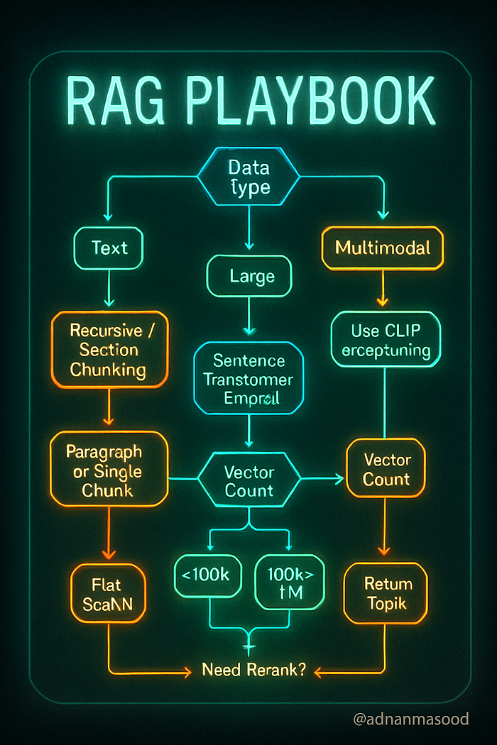
Choosing the appropriate chunking, embedding, and indexing strategy can be complex. The following is a decision flow (in Mermaid diagram format) to help guide decisions. It takes into account the data type (text vs multimodal), the complexity and size of the task, resource constraints, and retrieval requirements:

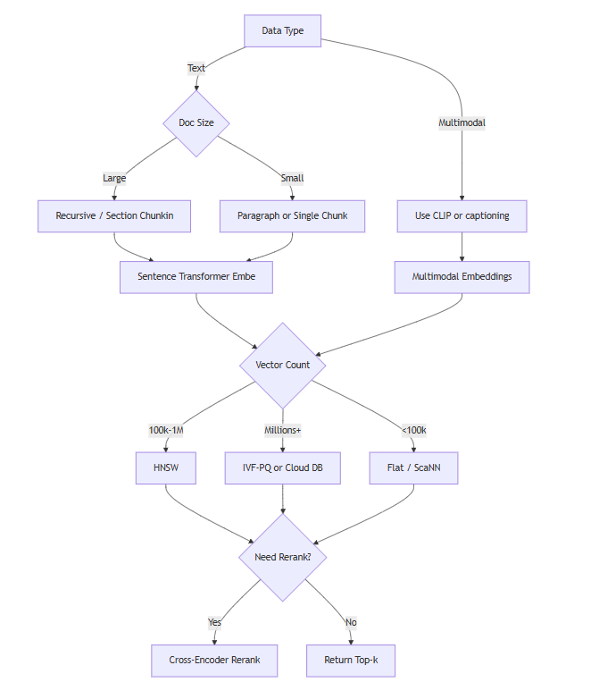
In the decision tree above:

• We start by determining if the data is purely text or multimodal. If multimodal, we incorporate the methods to handle those (like using CLIP or captioning). Regardless, we eventually chunk and embed into vectors.
• Then we consider embedding model choices based on resources. If we have limited compute (or need on-the-fly embedding for user-provided documents in a chat), a smaller model or an embedding API is preferable. If we can embed offline and quality is paramount, go for the best model you can (which might be slower).
• Next, depending on number of vectors, pick an indexing strategy: small data might not need fancy ANN, very large data might need a distributed solution.
• We check if we need metadata filtering (for example, user says "from 2021 documents only" or "only from source X"). If yes, ensure the chosen solution supports that easily (many open source vector DBs do; Faiss on its own does not have filtering logic, so you'd handle that separately).
• Finally, consider if a reranker will be used. If you have a strong embedding model and your results are already good, reranking may be overkill. But if you can afford some extra latency for improved precision, using a reranker like Cohere's ReRank (which is a model that given a query and a passage outputs a relevance score) or a cross-attention model can reorder the results so that the truly best chunk is on top. ColBERT, for instance, could re-score the top 100 via its late interaction mechanism. This often boosts answer quality in QA tasks at the expense of extra computation.
• The end of the flow is feeding into the LLM. That part involves prompt engineering (formatting retrieved chunks into the prompt properly, maybe with citations or tags).

This decision tree is a simplification, but it covers typical decisions. Real scenarios might loop back (e.g., if retrieval is slow, you might revisit using a smaller model or more aggressive ANN settings).

Compatibility with Different LLMs

One must also consider how the choice of chunking and embeddings interacts with the specific LLM used for generation, such as GPT-4, LLaMA, Claude, Gemini, or Grok:

• Context Window Sizes: LLMs like GPT-4 come in 8K and 32K context variants. Others like Anthropic's Claude have even 100K context versions. Meta's LLaMA-2 is around 4K by default, though there are finetuned longer versions. Google's Gemini is said to have enhanced long-context handling. For a smaller context model, you must keep chunks small and/or retrieve fewer chunks. A large context model theoretically lets you stuff more info (maybe you could skip chunking and pass a whole document if it's under 100K tokens), but beware: just because you can doesn't always mean you should. The larger the input, the slower (and costlier) the generation, and the model might still struggle to identify the relevant parts if you supply too much irrelevant text. So chunking is still valuable even with big contexts, to provide focused relevant info. But with something like a 100K context, you might retrieve 10–20 chunks instead of 3–5, improving recall for complex queries that need synthesizing many pieces.
• Tokenization differences: As noted, GPT-4 uses tiktoken (similar to GPT-3's BPE), LLaMA uses SentencePiece (where a chunk might have slightly different token count). It's not usually a major issue unless you are on a tight token limit. The bigger issue is if the embedding model and the LLM have different languages or text representations. For example, if you used a byte-level embedding model that is case-sensitive but the LLM lowercases everything internally (hypothetical), there could be mismatches. In practice, text is text — but if your LLM is trained primarily on a certain style of text, ensure your chunks are formatted in a palatable way (e.g., if the LLM sees a chunk with a lot of JSON or code and it's not a coding model, it might not handle it well).
• In-Context Learning vs Answer Extraction: Some LLMs (especially older ones) might not reliably use the retrieved info unless prompted well. Modern instruct-tuned models are generally good at it: e.g., GPT-4 will gladly incorporate any provided context. But if you use a base LLaMA model (not instruction-tuned) in a RAG setting, you need to prompt it carefully or fine-tune it to utilize retrieval. Fine-tuning an LLM on retrieval augmented tasks (like how RAG model from Facebook was trained) is an advanced approach — currently, most just do prompt-level integration.
• Public vs Private Models: If using a closed model like GPT-4 via API, you can't customize its internals — you rely on prompt engineering. If using an open model (LLaMA 2, etc.), you might fine-tune it to better handle the format of your chunks or even to embed documents itself (some people do a two-tower model with smaller LLMs). But fine-tuning 7B/13B models for embedding might not outperform just using a dedicated embedding model.
• Multimodal LLMs: Models like GPT-4 Vision or upcoming Gemini can accept image inputs directly. In a multimodal RAG scenario, you might not need to embed images as vectors at all — you could retrieve text via normal means, and separately if an image is needed, include the image file itself in the prompt (if the LLM can take an image file). For instance, if the query asks for a specific diagram and you have that image, a multimodal LLM could reason over it directly. However, current multimodal LLMs typically handle only a couple images in input, not a whole database. So you'd still have a retrieval step to find which image(s) to show the model, and that retrieval would likely use embeddings (like CLIP) as we described. In summary, a multimodal generation ability can replace the reading of the retrieved modality but not the retrieval step itself.
• Compatibility and Embedding Source: Some LLM providers (like OpenAI, Cohere) offer both the generation model and embedding model as part of the suite. Using embeddings from the same provider can sometimes have advantages — e.g., OpenAI might ensure their embeddings play nicely with their models' knowledge. However, there's no guarantee of that. It's more about convenience (same ecosystem). You can absolutely use SBERT embeddings and feed results to GPT-4 — it will work; the GPT-4 doesn't know or care how you found the text you gave it, as long as the text is relevant and well-formatted.
• Large vs Small LLMs in RAG: It has been observed that even smaller LMs (like 7B parameters) can give good answers if RAG provides the relevant text. In other words, retrieval can "boost" a weaker model by supplementing it with facts. If you plan to use an open-source model like LLaMA-2 7B or 13B to avoid API costs, putting a lot of emphasis on high-quality retrieval (maybe even more chunks, since the model's reasoning ability is lower) might be needed. Conversely, a very powerful model like GPT-4 might handle slight retrieval misses better (it might have some background knowledge to fill gaps or can infer missing bits). But relying on LLM internal knowledge is risky if you want factual accuracy, so always prefer giving it the exact info.

Reranking and Its Impact

Earlier we touched on rerankers like Cohere's ReRank model or ColBERT. These come into play after the initial vector search. They can significantly improve precision — for example, turning a top-10 list where 3 are relevant into a reordered list where the top 3 are those relevant ones, which means you can then feed fewer chunks to the LLM and still cover the answer.

How rerankers affect technique choice:

• If you decide to use a reranker, you might choose to retrieve more candidates (say top 50) from the vector index instead of top 5, because the reranker will shuffle them. The vector retrieval in this case is focused on recall (get all possibly relevant bits). This means you might tune your ANN index for slightly higher recall at cost of more results (maybe lower search pruning parameters). It also means more embeddings will be passed to the reranker, which is fine if reranker is reasonably efficient (Cohere's is fast, ColBERT is okay for tens of passages on CPU, or faster on GPU).
• Rerankers can compensate for less precise embeddings. Suppose you only have resources to use a smaller embedding model which sometimes brings in some off-target chunks. A reranker (especially a large cross-encoder like cohere ReRank or OpenAI's rerank via GPT-4 etc.) can often drop the irrelevant ones by truly understanding the query and chunk content deeply. So you might err on the side of wider recall with a simple embedder + powerful reranker.
• If using a reranker, you might not need as advanced an ANN index. Even something like "retrieve top 100 by BM25 and top 100 by embeddings, combine, then rerank with cross-encoder" is a viable strategy. It simplifies vector index needs (maybe you don't even need ANN if you can do small brute force on a subset). This hybrid approach is mentioned in various contexts. Qdrant's blog also notes combining vector search with rerankers for refined results.
• Cost of reranking: If using an API-based reranker (like hitting Cohere's rerank endpoint for each query), that's an additional inference cost per query. If using an open model cross-encoder like MS MARCO trained MiniLM, that's compute on your side. Ensure the latency is still acceptable when adding this step. Often it might add, say, 50ms to rank 50 passages with a small model, or a few hundred ms with a larger model. Some are okay with that for better answers.
• ColBERT in particular: It indexes multiple vectors per passage (one per term) and uses a late interaction scoring (max-sim of matching term embeddings). ColBERT v2 is efficient and can even be used as a first-stage retriever. But it complicates your pipeline (custom index structure). However, there are integrations (like LlamaIndex has a ColBERT retriever plugin). It can shine in scenarios where precise phrase-level matching is needed (like legal or technical QAs where a single term mismatch changes meaning; ColBERT would ensure the exact terms align, due to its max-sim mechanism focusing on exact contextual token matches). Using ColBERT as a reranker means you still do a vector search to get candidates (maybe with simpler embeddings), then use ColBERT to rescore.

When to skip rerankers: If your retrieval is already returning highly relevant chunks at rank 1 almost always (e.g., very targeted questions on a well-structured KB), the reranker might be overkill. Or if latency is critical and you rather feed 5 somewhat noisy chunks to the LLM and let the LLM figure it out. Modern LLMs are actually capable of pulling answer from a somewhat relevant passage even if a slightly more relevant one was slightly lower ranked (since you often include more than one chunk). But giving LLM too much irrelevant text can confuse it or cause it to include unrelated info. Rerankers help prevent that by only sending the good stuff.

Cohere ReRank example: It returns a relevance score and you can just sort by that. Very straightforward to use (as shown in LanceDB example).

Gotcha with rerankers: Ensure the text you feed into reranker is what you want evaluated. If you rely on metadata or title info to retrieve, include that for reranker too, if it influences relevance. Rerankers usually take the full text of chunk and the query, so if, say, a chunk is just "Section 2.1 … (then content)", you might want the reranker to see "Title: X, Section 2.1: content" if the title is needed to judge relevance.

In conclusion on reranking: It's a powerful add-on for quality, allowing you to use simpler chunking (maybe bigger chunks or less overlap) and still not lose precision, because the reranker will downweight any chunk that had extra fluff unrelated to query. It does add complexity and cost, so weigh it for your application.

Tools, Ecosystem, and Real-World Considerations

Finally, let's survey the landscape of tools and solutions, and talk about real-world performance and cost:

Tools and Solutions Overview

Open-Source Libraries & Frameworks:

• LangChain: An open-source framework that became popular for building LLM applications, especially RAG. It provides classes for text splitters (chunking), vector store integrations, embedding model wrappers, and chains that combine retrieval and LLM calls. LangChain supports many vector DBs as backends (FAISS, Pinecone, Chroma, etc.). It's great for rapid prototyping of RAG. For example, you can do VectorstoreIndexCreator with LangChain to auto-chunk, embed with a chosen model, and store in say FAISS – all in a few lines. It also helps orchestrate conversation memory, etc. The drawback is sometimes it can be a bit abstract or have performance overhead for very large data, but it's improving.
• LlamaIndex (formerly GPT Index): Similar purpose to LangChain, with a focus on index structures. It provides advanced features like tree-based indexes, keyword tables, and integration of rerankers (e.g., it has built-in support for using ColBERT or other rerankers). LlamaIndex can build indices that are beyond plain vector search (like a hierarchical index where the LLM first narrows by topics). This can be useful for certain use cases where pure vector search isn't enough or you want more interpretability.
• FAISS: We've discussed — it's a C++ library (with Python bindings) by Facebook for vector similarity search. It's kind of the gold standard for ANN benchmarking. Many production systems incorporate FAISS under the hood. It's open-source and highly optimized. If you need to roll your own on-prem vector search, FAISS is likely what you'll use (unless you opt for an all-Python library like Annoy or NMSLIB for simplicity with smaller data).
• Annoy: Open-source ANN by Spotify (C++ with Python). Good for simpler use cases, can persist index to disk. It's approximate and doesn't guarantee recall like HNSW can, but easy to use.
• ScaNN: Google's ANN library (in TensorFlow Recommenders), optimized for deep-learned vectors. It uses partitioning and quantization. Not as widely used as FAISS but has strong performance.
• Milvus: An open-source vector database (Chinese-origin, now part of Linux Foundation) that supports distributed deployment. It provides an interface (gRPC/python) to manage collections of vectors, with filtering, etc. Milvus under the hood can use Faiss or HNSW for the ANN part. It's a full server you run. If you need an on-prem solution that scales beyond one node, Milvus is a candidate.
• Qdrant: Another open-source vector DB (Rust-based). It offers a powerful query API with filters, payload (metadata) support, and implements HNSW (with quantization option). You can self-host it or use their cloud. Qdrant is known for being easy to use (HTTP API, or clients) and high performance. It also integrates with LLM frameworks (they have examples with LangChain, etc.). The Qdrant tech blog often writes about hybrid search and reranking topics.
• Weaviate: Open-source (in Go) vector DB with a lot of features: filtering, modular vectorizers (you can even have it call HuggingFace models for you to vectorize on the fly), and it supports hybrid search (BM25 + vector) natively. Weaviate uses HNSW index. It has a GraphQL API which some like. Also comes with a cloud offering. Weaviate can also store data in an eventually-consistent way with persistence.
• Chroma: A newer lightweight python vector DB (which LangChain initially bundled as default). Chroma is easy to integrate (just pip install, and it stores data locally in a SQLite under the hood). It's more for prototyping or small apps as of now, not a distributed system. But quite convenient.
• Elastic / OpenSearch: The well-known search engines also added vector search. Elasticsearch (from 7.5 onwards) has a vectors datatype and kNN search (via an plugin that uses HNSW). OpenSearch (Amazon's fork) has similar capabilities. They allow hybrid queries (BM25 + vector) and filtering since those systems excel at that. If you already have a search infrastructure, adding vector search to it might be attractive. However, these might not be as optimized for purely vector use cases as specialized DBs (for example, scaling to very large vector sets might be trickier or less cost-effective).

Proprietary and Cloud Services:

• OpenAI: Besides providing GPT-4, they provide the embeddings API. They don't (currently) provide a hosted vector database — that part you do yourself or via a partner. But OpenAI's influence is providing models (Ada embeddings, etc.) that many pipelines use. Also, the new function calling and retrieval plugins in OpenAI ecosystem allow an LLM to call a search API. For example, one could implement a tool where the LLM itself does the query to a vector DB (maybe via a plugin). This blurs lines — the LLM can decide what to retrieve. Exciting area but out of scope for now.
• Cohere: Similar to OpenAI, they have an embeddings API, a rerank API, and also generate models. They don't host your data, but their models are tuned for retrieval tasks (the Cohere Embed model, for instance, has multilingual options). Using Cohere Rerank can be an easy way to add reranking via API without hosting a cross-encoder yourself.
• Pinecone: A popular managed vector database service. You just push vectors (with metadata) and it handles indexing and searching via API. Pinecone abstracts whether it uses HNSW or IVF — but from their pricing page we deduce they have different pod types (some optimized for memory vs storage). Pinecone also automatically scales and shards. It's not open-source; you pay per usage. Great for not managing infra, but could get expensive if you have huge data (since pricing is by the pod/hour and number of pods needed is by vector count). Pinecone emphasizes low latency and ease of integration.
• Azure Cognitive Search: Azure offers vector search integrated into its Cognitive Search service. You can store vectors alongside traditional inverted indices and do hybrid queries. This is appealing if you want one service for both keyword and semantic search. Azure also has an "OpenAI" service to use OpenAI models within Azure. A typical Microsoft stack solution is: use Azure Cognitive Search with vector search for retrieval, and Azure OpenAI (GPT-4) for generation, all within Azure's ecosystem (data never leaving).
• AWS Kendra / OpenSearch: Kendra is Amazon's intelligent search service — originally more of QA over indexed docs (with some ML). They have added semantic capabilities. But one could also just run OpenSearch (which AWS manages, in ElasticSearch Service) with kNN plugin. Amazon also has Bedrock, which gives access to several foundation models (maybe use that for generation) and they likely envision usage with an AWS-native search.
• Google Vertex AI Matching Engine: Google Cloud offers a managed ANN service called Matching Engine, which uses Google's ANN tech (ScaNN, etc.). If your data is on GCP, that's an option. They also have Vertex AI Generative (PaLM, etc.), so similar to Azure one could stick within one cloud for both retrieval and generation.
• Other cloud DBs: There's many startups: Pinecone, Chroma Cloud, Weaviate Cloud, Qdrant Cloud, Redis (Redis Stack has vector similarity search module, and Redis Enterprise Cloud can host it), Milvus-powered Zilliz Cloud, etc. Each has different pricing and slight feature differences (e.g., some focus on ease of use with certain ecosystems, some on hybrid queries, etc.). The vector DB comparison we attempted to see gave a rough idea: FAISS fastest (but not a service, just library), Qdrant, Pinecone close. Weaviate, Milvus also in mix. Chroma is more local usage for now.

Benchmarks:

• BEIR (2021): We've referenced it. It provided a benchmark to test retrieval on many datasets. It compared BM25, USE, SBERT, etc., and cross-encoders. The result was: cross-encoders (rerankers) did best but slow; BM25 is surprisingly strong in zero-shot; dense embeddings vary — some beat BM25 on some sets, but not all; and hybrids often did well. This benchmark pushed development of better embedding models (e.g., multifacet tuning to cover diverse tasks).
• MTEB (2022/2023): Massive Text Embedding Benchmark. This is like BEIR but broader (58 datasets, including not just retrieval but clustering, classification tasks too, and multilingual aspect). The finding that "no one model dominates all tasks" suggests that for your specific use case, you should choose a model that's known to do well on similar tasks. MTEB's leaderboard shows models like E5-large, Instructor-XL, GTE-large, etc., performing very well on retrieval sub-scores. If your use case is close to, say, QA or web search, those are indicative.
• MS MARCO (2018 onward): This is a dataset of Bing search queries and passages; it spawned a leaderboard that drove a lot of progress in retrieval. Many dense and reranker models were first benchmarked on MS MARCO. It's not zero-shot (models train on a train set). But a lot of techniques (like knowledge distillation from cross-encoder to bi-encoder) were developed to maximize MARCO metrics. The takeaway: the top bi-encoder retrievers can reach ~.40 MRR\@10 on MS MARCO (while cross-encoders can be ~.42). These numbers aren't directly meaningful for everyone, but it shows dense retrieval can get close to cross-encoder if trained well. If you have your own training data, you can achieve very high accuracy retrieval with a custom model, otherwise you rely on these general models.

Real-World Performance and Cost

Let's talk practical numbers and experiences:

Latency: For a well-optimized ANN (HNSW) in memory, searching 1 million vectors can be on the order of a few milliseconds for top-10, if the index is in RAM and you have enough CPU. HNSW can do 100–200 queries per second per CPU core in some cases. If you use a service like Pinecone, a single p1 pod (1 replica) might handle around that magnitude (depending on vector dim). If you need more QPS, you add more pods (they'll shard or replicate as needed). The aimultiple report mentioned Zilliz (Milvus) having the best raw latency, with Pinecone and Qdrant also competitive, for 1M vectors. The differences are often small if all using HNSW.

For disk-based (like if data doesn't fit RAM and using IVF-PQ with paging from disk), latency might go to tens of milliseconds or more, depending on how many disk pages need to be loaded. Systems like Vespa or Lucene's ANN try to memory-map data so the OS cache handles it.

Throughput: If you have concurrent queries, throughput matters. Pinecone and others rate-limit or suggest how many QPS a pod can handle. E.g., a p1.x1 (small) pod might handle ~50 QPS for moderate d and still <100ms each. If you exceed that, you get queueing or you scale out.

Scalability: Most vector DBs can handle tens or hundreds of millions of vectors by sharding across machines. But costs escalate linearly with shards. If each machine can do 5M vectors comfortably in RAM, for 100M you need 20 machines, etc. This is where cost vs performance trade-offs come in: compress vectors to fit more per machine or accept slightly higher latency for a multi-hop search.

Memory usage: It's often the biggest cost. Storing 100M 768-d float32 vectors = 300 GB. In practice, you'd use compression (like 8 bytes per vector with PQ, cutting that to 100M * 8 = 800 MB, much nicer with some accuracy loss). Or store on SSD and read on demand (slower but cheaper). Cloud services usually charge by the RAM or by vector count which implicitly covers their infra cost.

Cost comparison of tools: Open source ones you pay for hardware. Cloud ones you pay usage. A quick example: Pinecone's pricing (as of reference) for 1M vectors on a 1x pod is ~\$0.111/hour (for performance tier) — that's ~\$80/month. If you have 10M vectors, you'd need either a bigger pod or 10x pods, so ~\$800/month. Weaviate Cloud or others have different pricing (some charge by data GB, or by cluster size). If self-hosting on cloud VMs, cost is just VM cost + your time.

Real-world throughput example: Suppose you have a support chatbot that gets 5 queries per second, each query embedding and retrieval in 50ms, and an LLM call 1000ms. That's fine. If you have a public-facing search for a website with 50 QPS, you'd likely need to optimize/horizontally scale.

Example performance (hypothetical based on references and experience):

• A single CPU core using Faiss Flat L2 on 100k vectors of dim 384 can do ~1–2ms per query for top-10.
• HNSW on 1M vectors dim 384 might do ~5–10ms at 95% recall on 1 core (ef=100, M=32). Multi-threading can reduce wall time further (Faiss by default uses multiple threads if you enable).
• On GPU, brute force 1M x 384 maybe ~<10ms as well with a good GPU (because 1M*384 ~ 384e6 operations, which a GPU can handle easily).
• Rerank with MiniLM cross-encoder on 50 candidates: ~50ms on CPU.
• Rerank with a bigger model (like MPNet cross-encoder): ~200ms on CPU, or much faster on a GPU if available.

Handling scale: Companies like Google or Bing obviously operate at billion-scale documents. They use multi-stage retrieval (first cheap sparse to narrow to thousands, then vector search on a smaller set, etc., plus heavy caching). In a smaller domain RAG (say enterprise documents), our scale is usually smaller and simpler.

Monitoring costs: If using OpenAI for embeddings and GPT, your major cost might ironically be the GPT calls, not the vector search infra. But if you have a lot of data, the embedding step initially could cost more (embedding a million docs might cost ~\$400 with Ada). Pinecone or others start adding up if you keep a lot of data live. Some projects opt to periodically load/unload indices or only index a subset (like most recent docs) to control costs.

Example Use Cases (putting it all together):

• Customer Support: A chatbot that answers support questions by retrieving knowledge base articles. Likely chunk by FAQ or by paragraph in help docs, embed with a general model (or a support-finetuned MiniLM if available), store in a vector DB (maybe with sections like "product area" as metadata). When a user asks something, retrieve a few relevant snippets and either directly return or feed to an LLM to compose a nice answer. This reduces load on human agents and ensures answers are grounded in official documentation (reducing hallucinations). The system must be able to search by error codes, product names (so incorporate those terms well in embeddings or fallback to keyword if needed). Reranker might be used if queries are verbose (to pinpoint exact answer).
• Legal Document Analysis: Lawyers have a huge repository of contracts and case law. RAG can help by retrieving relevant clauses or past cases given a query. Here, chunking is critical: legal docs have sections and definitions; chunk by clauses so that retrieval can find a specific clause (e.g., "termination clause"). Possibly use a model like LegalBERT or CaseLaw-BERT for embeddings to understand legal language nuances. Because exact terminology matters, one might do hybrid: ensure exact term matches (like a specific law number) are not missed by also doing keyword search. The LLM (maybe GPT-4, since it's good at understanding complex language) then gets relevant clauses to answer a question like "Can party X terminate the agreement early under Y clause?". Privacy is a concern here, so likely an on-prem solution (maybe self-hosted Qdrant or FAISS) with an open LLM or an Azure OpenAI in a secure environment.
• Academic Research Assistant: A tool for researchers to query a corpus of academic papers (like semanticscholar or arXiv). It could allow questions like "What are recent developments in graphene-based solar cells?" The system would chunk papers by abstract, introduction, conclusions, etc. and embed them (maybe using SciBERT or Specter embeddings specialized for academic citations). Vector search finds relevant passages across many papers. Possibly rerank by a criterion like publication date or citation count if user wants the latest or most influential. The LLM (maybe fine-tuned for summarization) then summarizes or gives an answer citing those works. The challenge here is volume (hundreds of thousands of papers) and multi-lingual or formula content in some fields. Vector search handles synonyms (e.g., "graphene-based solar cells" vs "graphene photovoltaics"). One must be careful with chunking equations or figures (perhaps treat them as separate chunks with their alt text or captions).
• Real-Time Applications: Some RAG uses involve real-time data, e.g., a bot that can answer about the latest news. That requires continuously ingesting new documents and chunking/indexing quickly (streaming into the vector store). Many vector DBs support upserts in real-time. The embedding model should be fast (maybe use a smaller model if needed to embed streams of data quickly). The LLM might also need to be updated or at least not contradict if it has training data that says something else (one reason retrieval is used, to override outdated info).
• Code search: Another interesting use case — embedding code snippets for natural language search (like "How to parse JSON in Python?" retrieving code examples). You'd chunk code by function or snippet, embed using code-aware models (like CodeBERT or UniXcoder). The index might be millions of code snippets (GitHub etc.). For search, you might combine text and code search: query might match a code comment or function name (embedding catches that) or specific API usage (embedding also can catch that if trained on code). If LLM is used (like to explain the retrieved code), that's more of generation. A caution: code tokens are different distribution; specialized models help because generic models might not differentiate json.loads vs json.dumps well in vector space.

Security and Privacy: In real deployments, consider access control — e.g., a vector DB that can filter results by user permissions (metadata filtering by user or group). This is crucial if using RAG on private data with multiple users. Some enterprise solutions (like Azure Cognitive Search) integrate with AD for that. If building from scratch, you'd have to enforce filters on queries.

Evaluation: Finally, test your RAG system with real queries and measure answer quality. Tools like LangChain provide evaluation harnesses. You want to ensure that for known query-answer pairs, the system retrieves the supporting info and the LLM answers correctly using it. If not, adjust chunk size or embedding model or add more data, etc. RAG has lots of moving parts, so a failure could be in retrieval or in generation — isolating which is key. If retrieval is failing, maybe add data or improve embeddings. If generation is failing (e.g., not using the retrieved info properly or style issues), adjust the prompt or the LLM choice.

Tables for Tool Comparison

We include two LaTeX tables below: one comparing chunking strategies/tools and one comparing some vector database options, to provide an at-a-glance reference.

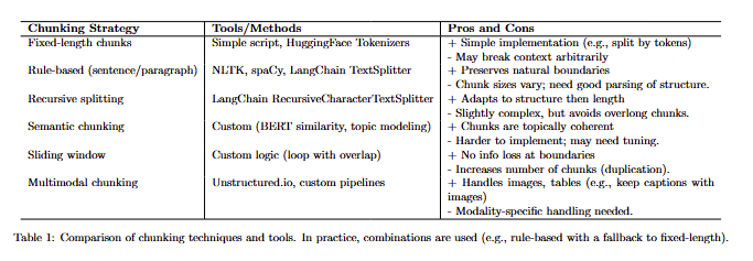
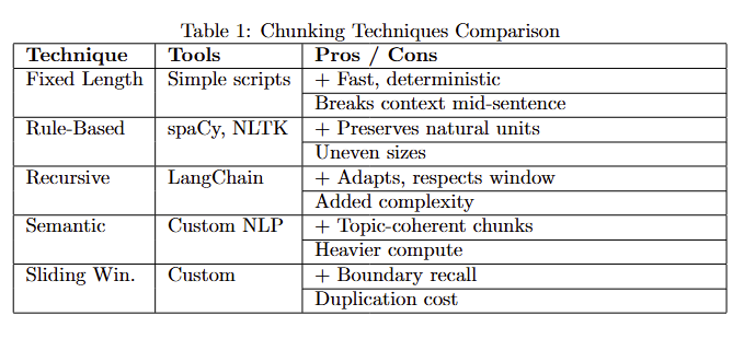
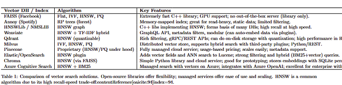
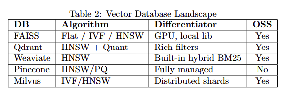
Table 2: The table illustrates that many vector search solutions use similar core algorithms (HNSW, IVF), but differ in features (filtering, scaling, ease of integration). Open-source options like FAISS or Qdrant allow on-premises deployment and customization, while cloud services like Pinecone or Azure provide convenience at a cost. The choice often depends on requirements for scaling, real-time updates, integration with existing stack, and budget.

Real-World Use Cases

To ground these concepts, let's revisit a few real-world scenarios and see how the strategies come together, highlighting any unique considerations:

• Customer Support Assistant: A large company deploys an AI assistant to help answer IT support tickets and questions using an internal knowledge base. They chunk the knowledge base articles by FAQ or paragraph (using a rule-based splitter, ensuring each Q\&A pair stays intact). They use a medium-sized embedding model (MiniLM) to keep latency low, since they have many concurrent users. The embeddings are indexed in Qdrant with HNSW. When a user asks a question, the system retrieves the top 5 relevant chunks. They noticed that sometimes multiple chunks from the same article come up; to avoid repetition, they group by document so the final answer covers diverse sources. They feed the top results to GPT-4 with a prompt like: "Answer the question using the info from these excerpts." This system helped deflect a significant portion of support queries by providing instant answers, with sources quoted (they include the document title from metadata in the prompt so GPT-4 can say "According to [Document] …"). A pitfall they overcame: initially, the model sometimes gave outdated info because some chunks were from older docs. They added a metadata filter to prefer chunks from the latest policy documents (or added "date" as metadata and in the prompt instruct GPT-4 to prioritize newest info). This improved the relevance of answers.
• Legal Contract Analysis: A law firm uses RAG to analyze clauses across thousands of contracts. They chunk contracts into clauses (leveraging the fact that contracts have numbered sections). They use a Legal-BERT based sentence transformer for embeddings to capture legal terminology nuances. For a given query (e.g., "show all force majeure clauses that mention 'pandemic'"), the system does a vector search to find semantically similar clauses, then applies a keyword filter for "pandemic" to narrow results. It outputs the clauses to an interface for the lawyer to review, with the relevant terms highlighted. Here, they actually didn't use an LLM to generate answers, because the lawyers prefer to read the actual clauses. Instead, it's a pure retrieval use case. But they did use an LLM offline to cluster similar clauses (like grouping all pandemic-related force majeure clauses) to help create a summary report. A challenge was ensuring confidentiality — they ran the entire pipeline on-prem, using open-source tools (HNSW index via FAISS) and a self-hosted LLM (they fine-tuned LLaMA on legal text for any generation tasks). They also had to deal with OCR errors in older scanned contracts; those made some embeddings garbage, so they implemented a confidence check on text quality (if OCR output had too many unknown tokens, they skipped those chunks).
• Academic Literature QA: Researchers built a system where you ask a question and it finds answers from academic papers. For example: "What experimental setups have been used to increase solar cell efficiency?" The system chunked papers by sections and also by sentences (for fine-grained search). It uses a strong embedding model (Instructor-XL) which was top on MTEB for science QA. The vector index is Milvus in cluster mode because they have 5 million chunks (from about 50k papers). When a question comes, it retrieves 10–20 short excerpts (sentences or paragraphs) that might contain an answer. They feed these into an LLM (Claude with 100k context in this case) which then writes a summary answer citing each source. Because of the long context, they actually include more chunks than a smaller context model would allow, improving completeness. One pitfall: sometimes different chunks had conflicting info — the LLM initially merged them incorrectly. They solved this by prompting the LLM to provide multiple possible answers if evidence diverges, or by using a reranker to only pick the top 5 most relevant and consistent chunks. They measured answer accuracy by comparing to human-written answers on a set of test questions and found it to be very high, showing the importance of good retrieval.
• E-commerce Search and Recommendation: A retailer uses embeddings to improve product search on their website. They chunk product descriptions by sentence. They index both the text and image embeddings for each product (using CLIP). When a user searches with a text query, they do two searches: one in text embedding space, one in image embedding space (treating the query text as CLIP text embedding for the image index). This way, even if the text description lacked a keyword, a product image that semantically matches might surface (e.g., query "floral summer dress" might find an image of a dress with a floral pattern even if the text didn't say "floral"). They combine these results in a merged list. They also use the vector similarity between products to power a "similar items" recommendation widget. The vector store is Pinecone for ease of scaling with their growing catalog. They do have to retrain or update embeddings when new products arrive, but since that's continuous, they built a pipeline to update Pinecone incrementally each day. A key learning for them: product titles are short and sometimes not descriptive, so they included not just description but also user reviews text (aggregated) as part of the chunk content to enrich the embeddings. This yielded better search results, because sometimes users search with terms that appeared only in reviews (e.g., "durable" or "good for small apartments").

Through these examples, it's clear that the combination of chunking, embedding, and vector search must be tailored to the data and the problem. The strategies we've discussed provide a toolbox to draw from.

Conclusion

In this article, we covered the full spectrum of Retrieval-Augmented Generation (RAG) technical components:

• We defined chunking, embedding, and vectorization in RAG and why each is essential, including handling of multimodal data.
• We explored chunking techniques from simple fixed-length to advanced semantic chunking, with code examples and use cases for each.
• We surveyed embedding methods, from Word2Vec and GloVe to BERT-based models and CLIP for images, discussing their evolution and usage, and provided practical code and advice.
• We detailed vector index strategies like HNSW and IVF, and optimizations like normalization, PQ, and discussed how to choose an approach depending on scale.
• We looked at history and milestones (BERT, SBERT, CLIP) that led to current best practices, and enumerated best practices (and common pitfalls) in implementing these systems.
• We provided a decision tree to guide selecting methods under various constraints, and examined compatibility with different LLMs (context lengths, etc., including emerging ones like Gemini and Grok with very long contexts).
• We analyzed the role of rerankers like Cohere ReRank and ColBERT, noting how they can improve final results and what trade-offs they bring.
• We surveyed the ecosystem of tools (LangChain, FAISS, Qdrant, Pinecone, etc.) and benchmarks (BEIR, MTEB, MS MARCO) to contextualize these techniques in real-world systems.
• Finally, we looked at real-world performance considerations and walked through concrete use cases integrating all these components, demonstrating how theory translates into practice.

The field is moving fast — new LLMs with larger context and new embedding models are emerging — but the core principles of RAG remain: break the knowledge into pieces, represent those pieces in a way the machine can reason with, efficiently find the pieces you need for a given query, and feed them to a generative model to produce a grounded response. By following the strategies and best practices outlined here, practitioners can build RAG systems that are robust, accurate, and efficient for a wide range of applications, from question answering to search and beyond. With careful consideration of chunking granularity, embedding selection, and indexing techniques, as well as awareness of tools and their capabilities, one can avoid common pitfalls and create a system that truly augments an LLM's capabilities with the wealth of external knowledge available.

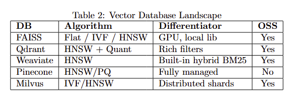
References and Further Readings

Word2Vec (2013) → https://arxiv.org/abs/1301.3781 GloVe (2014) → https://nlp.stanford.edu/pubs/glove.pdf BERT (2018) → https://arxiv.org/abs/1810.04805 Sentence-BERT (2019) → https://arxiv.org/abs/1908.10084 DPR (2020) → https://arxiv.org/abs/2004.04906 CLIP (2021) → https://arxiv.org/abs/2103.00020 BEIR Benchmark (2021) → https://arxiv.org/abs/2104.08663 MTEB (2023) → https://arxiv.org/abs/2210.07316 FAISS Library → https://github.com/facebookresearch/faiss HNSW Paper → https://arxiv.org/abs/1603.09320 Pinecone Docs → https://docs.pinecone.io Qdrant Docs → https://qdrant.tech/documentation Weaviate Docs → https://weaviate.io/developers LangChain Repo → https://github.com/langchain-ai/langchain LlamaIndex Repo → https://github.com/jerryjliu/llama_index Cohere ReRank → https://docs.cohere.com/docs/rerank ColBERT Paper → https://arxiv.org/abs/2004.12832 OpenAI Embeddings → https://platform.openai.com/docs/guides/embeddings Instructor Embeddings → https://github.com/HKUNLP/instructor-embedding E5 Embeddings → https://arxiv.org/abs/2206.01883