


This is the final article in the survival analysis series, where I will cover the last technique mentioned in the first episode of the series: Cox Regression. If you want to review the previous articles in the series, you can find them in the resources section.
As always, if you find my articles interesting, don't forget to clap and follow 👍🏼, these articles take times and effort to do!
What is Cox Regression and Hazard Ratio ?
Cox Regression : Also known as the proportional hazards model, it is a semi-parametric model used in survival time analysis to assess the effect of several variables (also called covariates) on the time until a specified event occurs.
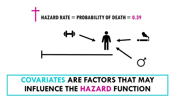
1 — Hazard rate and covariates : Also known as the Hazard, is the rate at which events occur, given that the individual has survived up to a certain time "t". This hazard rate is influenced by covariates, with each covariate having an associated coefficient that provides the hazard ratio for that covariate (I will explain everything)
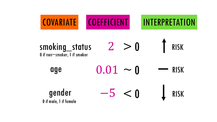
Interpretation of the coefficient :
- Positive Coefficient (β>0): Indicates that as the value of the covariate increases, the hazard increases.
- Positive Coefficient (β around 0): Indicates no difference in the hazard.
- Negative Coefficient (β<0): Indicates that as the value of the covariate increases, the hazard decreases.
Note : The magnitude of β gives the strength of the effect of the covariate on the hazard rate. Larger absolute values of β indicate a stronger effect.
For example, if a covariate like smoking has a coefficient (β) of 0.1, it means that a one-unit increase in the covariate (smoking one additional pack per day) is associated with a 0.1 increase in the log hazard of the event (Death).
To make this easier to interpret, we exponentiate the coefficient to obtain the Hazard Ratio.
2 — Hazard Ratio : There is also an important concept related to Cox Regression called "Hazard Ratio" which is the exponentiated coefficient
In the continuity of the previous explanation : The Hazard Ratio was exp(0.1).
Calculating this, we get exp(0.1)≈1.105. This means that a one-unit increase in the covariate (example ; smoking one additional pack per day) is associated with a 10.5% increase in the hazard of the event occurring. Better, right?
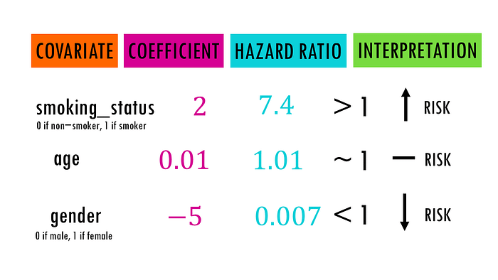
Interpretation of Hazard Ratio :
- A hazard ratio of 1 indicates no effect
- Greater than 1 indicates increased risk
- Less than 1 indicates decreased risk.
Why Exponentiate the Coefficient?
- Non-Negative Hazard Rate : By exponentiating the coefficients, we ensure that the hazard ratios are always positive, which aligns with the requirement for hazard rates.
- Interpretation : The exponential of the coefficient (exp(β)) gives us a hazard ratio, which is easier to interpret.
Mathematical representation of Cox Regression

- h(t): Hazard function at time t
- h0(t): Baseline hazard function
- β1,β2,…,βp: Coefficients of the predictor variables
- X1,X2,…,Xp: Predictor variables
Let's have an example to understand
We have a dataset of patients with a certain medical condition. The patients were treated with either Treatment A or Treatment B.
We want to use Cox regression to analyze the impact of treatment type, age, and gender on the survival time of the patients.
1 — Creation of the data : Like previous example I will use Numpy to create a data for 100 patient, and provide a seed for reproducibility if needed
- Age will be around 60 with a standard deviation of 10.
- Gender: Random choice between male and female.
- Treatments: Either the first or the second (0: Treatment A, 1: Treatment B).
- Simulate survival times in days with Treatment B having longer survival.
- Simulate events and combine everything in a DataFrame.
np.random.seed(42)

n_patients = 100

ages = np.random.normal(60, 10, n_patients).astype(int)
genders = np.random.choice([0, 1], n_patients)

treatments = np.random.choice([0, 1], n_patients)


base_hazard = 0.02
time_A = np.random.exponential(scale=1 / base_hazard, size=n_patients)
time_B = np.random.exponential(scale=1 / (base_hazard * 1.5), size=n_patients)

survival_times = np.where(treatments == 0, time_A, time_B)

events = np.random.binomial(1, 0.8, n_patients)

data = pd.DataFrame({
    'age': ages,
    'gender': genders,
    'treatment': treatments,
    'time': survival_times,
    'event': events
})

data.head()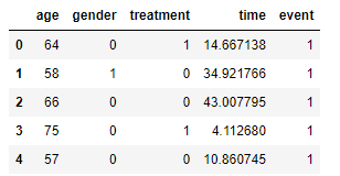
2 — Fitting the Model : Similar to the Meier curve example, we will fit the model in two lines of code and print a summary (including the p-value)
cph = CoxPHFitter()
cph.fit(data, duration_col='time', event_col='event')

cph.print_summary()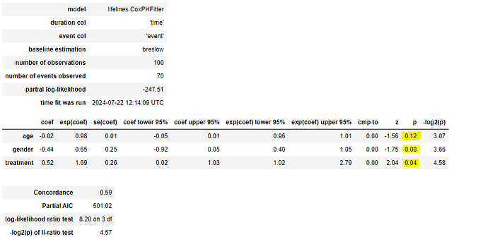
From the summary, we can observe the coefficient related to each covariate and the hazard ratio(which is the exponent of that coefficient).
The treatment is the only statistically significant covariate. According to the cmp value of "0" ,Treatment A increases the risk of events by 64% compared to Treatment B.
The other parameters are :
Standard Error of the Coefficient : measures the precision of the coefficient estimate (a smaller standard error indicates a more precise estimate of the coefficient)
- For example age has 0.01 se(coef) meaning the estimated coefficient could vary by 0.01 units in repeated samples.
Confidence Interval Bound : representing the lower and the upper bound of the 95% confidence interval for the coefficient (provides a range within which the true coefficient is expected to lie with 95% confidence)
- Always same row, for example the coef lower 95% of age is — 0.05, it means we are 95% confident that the true coefficient is at least — 0.05
Comparison to a Reference Category : In categorical variables, this indicates the reference category against which other categories are compared.
- In our case : (0: Treatment A, 1: Treatment B)
Z-Statistic : This is the test statistic used to test the null hypothesis that the coefficient is zero.
P-Value : A small p-value (typically < 0.05) suggests that the coefficient is significantly different from zero rejecting the Null Hypothesis, In our case only Treatment is significant with a p-value of 0.04
If there's a specific subject you'd like us to cover, please don't hesitate to let me know! Your input will help shape the direction of my content and ensure it remains relevant and engaging😀
Resources
Introduction to Survival Analysis
Log Rank Test for Survival Analysis
Kaplan Meier Curve
Please consider the following and subscribe to the newsletter for more articles about business, data science, machine learning, and extended reality, it's FREE! You can find my lists in the following links :
- Data Science Digest : https://medium.com/@soulawalid/list/statistics-data-science-65305693779d
- Generative AI : https://medium.com/@soulawalid/list/generative-ai-ee31117869a9
- Programming with Python : https://medium.com/@soulawalid/list/programming-c0a3ef000f5f
- Linguistic AI Lab : https://medium.com/@soulawalid/list/linguistic-ai-lab-9eb7d30369c1
- Strategic Business Intelligence : https://medium.com/@soulawalid/list/strategic-business-intelligence-1528f08575a7
- AI for Health Professionals : https://medium.com/@soulawalid/list/ai-for-health-professionals-f8b87eeab19f
- The Neuroscience of Consumer Behavior : https://medium.com/@soulawalid/list/the-neuroscience-of-consumer-behavior-8f94149e3c73
- Beyond Reality : https://medium.com/@soulawalid/list/beyond-reality-bf03607b0b80
- Quantum Leap : https://medium.com/@soulawalid/list/quantum-leap-be0b06f7a986
If you have any questions, you can ask me on LinkedIn, here is my profile: https://www.linkedin.com/in/oualid-soula/ Let's connect!