
We may have formalized mathematics and possess excellent computational tools in the modern era, but human ingenuity that created some of these mathematical ideas dates back to over 2000 centuries. Archimedes in 3rd century BC preseted a method to compute the value of pi to any required precision by repeatedly doubling the sides of the polygons inscibed within the circle. Already during 6th century BC, we know from Pythogoras that the squared length of the hypotenuse of a right angle triangle is the sum of the squared lengths of the sides. Image below shows a simple proof.

We can easily see that the area (or perimeter) of the circle can be bounded by that of a square inside whose vertices touch the circle, and an outer square whose sides are tangents to the circle. This gives the lower and upper bound for pi to be 2*sqrt(2) and 4.
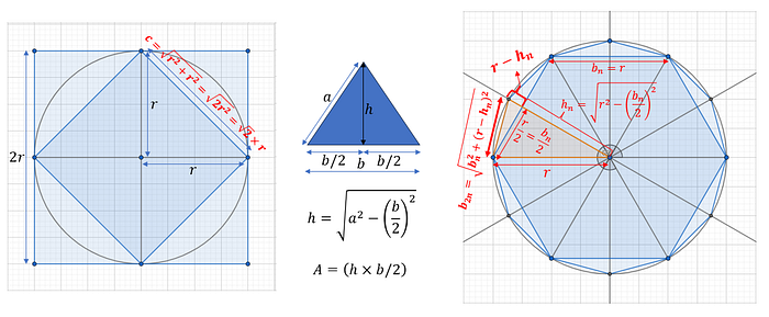
Archimedes realized that he can inscribe a n-sided polygon within the circle and by repeatedly doubling the n, he could approximate the circle's perimeter with increasing accuracy. We can see in the image above how the length of the sides are calculated when we go from the 6-sided hexagon to the 12-sided polygon. Each of the 6 triangles on the hexagon are isosceles and the height can be calculated via the pythogoras theorem. The base of the 12-sided polygon can be calculated using half the base of the 6-sided polygon and the height of the new right angle triangle that is the difference between the radius and the height of the 6-sided polygon. These relationships hold everytime we double the sides of the polygon and gives us a recursive relationship that gets us closer and closer to pi.

One radian is defined as the angle subtended at the center of a circle by an arc whose length is equal to the circle's radius. The are 2π radians in the circle and since each radian corresponds to the arc length r, the perimeter of the circle is 2πr. The arclength is r for 1 radian, and 2πr for pi radians. For any angle θ measured in radians, the arclength is θ×r.
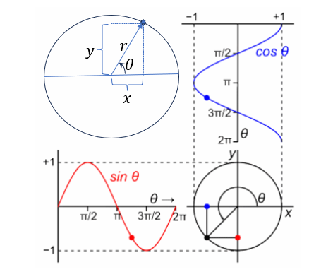
The circle gives rise to the sine and cosine functions, as shown in the image below. As we increase the angle, the x-coordinate of the point on the circle traces out the cosine function and the y-coordinate of the point traces out the sine function.
Aryabhata, the 5th century Indian astronomer (all mathematicians were astronomers then) knew how to calculate sine for specific angles and compiled a table of sine values in increments of 3.75 degrees. In 7th century, Brahmagupta refined the sine table using a second order (parabolic) interpolation that utilized his method of finite differences.
Brahmagupta also generated formulas for the sum of powers of first n natural numbers by considering the sum S(n) to be a polynomial of a certain degree. The polynomial order was found by checking the the first difference ΔS(n) = S(n+1)-S(n) for different values of n, the second difference Δ²S(n) = ΔS(n+1)-ΔS(n) for different values of n and so on, until the kth order difference that results in a constant for all n. This approach closely resembles differentiation, where the kth derivative of a polynomial of degree k is a constant.
For example, the sum S(n) = 1²+2²+…+n² can be represented by a polynomial of degree 3: S(n)=an³+bn²+cn+d. The coefficients can then be found by evaluating S(n) for different values of n and solving the system of equations. Of course it wasn't done exactly this way by Brahmagupta since the language and notations of mathematics in those days were very different from the modern notations we use today.

Another 700 years later, Madhava of Sangamagrama (from present-day Kerala) developed an ingeneous method of computing the infinite series expansions of sine and cosine. His method, in similar spirit as that of Archimedes, uses recursive refinement of an initial approximation by relying just on geometric principles, the only tools available at that time for doing mathematics. Image below shows the geometric construction that enabled Madhava to clevely apply recursion.
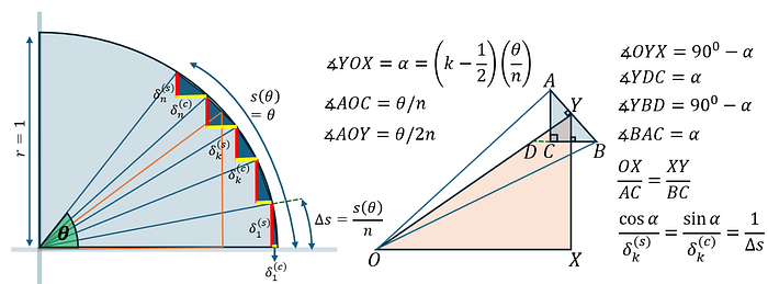
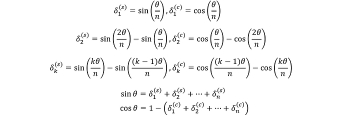
For an angle θ on the unit circle, the arclength s(θ) equals θ (since radius is 1). This angle can be divided into n equal parts, and the arclength for each part is then θ/n. The chords on each of these equal segments forms the hypotenuse of a right angled triangle. The sine of the angle θ is then the sum of all the red lines in the figure, and the cosine of θ is 1-sum of all the yellow lines in the figure. We can write the lengths of the red lines and yellow lines as shown in the equations below.
Take one of these arc segments and construct an angle bisector OY that intersects the chord AB at its midpoint Y. We now have two similar triangles BAC and XOY, because the angle XOY is same as the angle CAB. The ratio of sides of the similar triangles must be same and this gives us something that looks like a derivative formula, a full 300 years before Newton developed differential calculus!

These techniques used by Indian mathematicians way before the ideas being rediscovered in Europe is the cause for some claims that calculus was invented in India and later stolen by Europe. See this article for related details and references. We don't have to get into that argument and it is a topic best left to historians — here is an excellent set of slides on the history of trignometry in India by Professor K. Ramasubramanian of IIT Bombay.
Even the method of exhaution that Archimedes used to compute area closely resembles how we do integration, so ancient mathematicians had some intuition about the underlying ideas of calculus. Therefore, regardless of who gets the final credit, we can always marvel at the ingenuity involved to arrive at some of these results. Let us continue with our narrative.
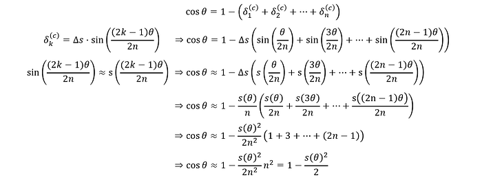
Madhava started with the the summation expression for cosine, used the approximation that sin(θ) for small values of θ is very close to its arclength s(θ), and derived the first order approximation cos(θ)≈1-θ²/2. In the derivation, he made use of the result that was already well known during Euclid's time (300 BC), that the sum of odd numbers 1 + 3 + … + (2n-1) is n².
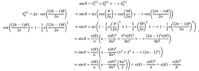
Madhava then substituded this approximation for cos(θ) in the equation for sin(θ) to get another approximation: sin(θ)≈θ-θ³/3. Thanks to the work done by Brahmagupta, the formulas for summation of other powers of odd numbers were also known and Madhava needed them for deriving these approximations.
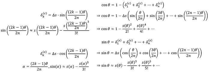
He could now do this recursively, by using the new approximation for sin(θ)≈θ-θ³/3 to get refined approximation for cos(θ), then use that back into the sin(θ) expression to improve the approximation and so on. This can be continued ad infinitum to get the infinite series expansion of sin(θ) and cos(θ). Remember that in all these equations s(θ) = θ×r = θ since r = 1.
Again, remember, dear reader, that the derivations presented herer use our moderm mathematical notations and the original work by Madhava was written in a very different formulation. It took a lot of work by different authors to interpret and express that in our modern notation. This particular proof I present here was gathered from this youtube video. There is also another interesting way to derive this infinite series expansion using involutes (as seen in this video.)
The expansion for tan(θ) = sin(θ)/cos(θ) can be computed via polynomial long division: (θ-θ³/3!+θ⁵/5!+…)/(1-θ²/2!+θ⁴/4!+…)=(θ+θ³/3+2θ⁵/15+…)
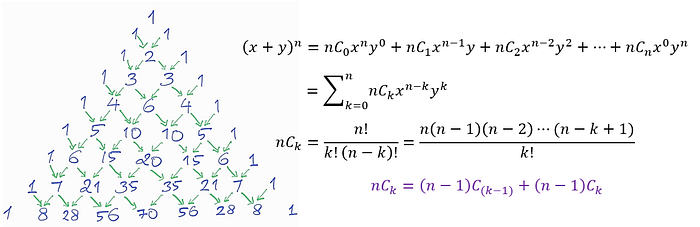
Another 300 years later, Newton when looking at expressions of the form (1+x)^n, wondered if the binomial expansion can be extended for fractional n. While the binomial coefficients were known in some form as early as 200 BC to Indian mathematician Pingala, it was systematically studied by Pascal only in the 17th century. For (a+b)^n, the terms of the binomial expansion are of the form (a^(n-k))(b^k) and the binomial coefficients nCk represent the number of unordered ways in which we can choose k number of b out of n. Pascal's identity shows that the kth coefficient on the nth row (expansion for power n) is the sum of the (k-1) and kth coefficients of the (n-1)th row (expansion for power n-1). It is easy to verify that this is true by writing out the fractions and simplifying them.
As an interesting tidbit, in his Sherlock Holmes stories, Sir Arthur Conan Doyle describes Professor Moriarty as a criminal mastermind with an exceptionally brilliant mathematical mind who authored a treatise on the Binomial Theorem when he was just 21. Perhaps this would intrigue some of you, dear readers, to read about the adventures of Sherlock Holmes, which in my opinion is a must read for engineers.
The deductive reasoning of Sherlock Holmes offers a fresh perspective on how to approach problem-solving — breaking problems down, collecting clues, assembling pieces of the puzzle, and realizing that more are needed before the full picture emerges, then do what is required to find those pieces. When you have eliminated the impossible, whatever remains, however improbable, must be the truth. Even problems that seem impossible at first turn out to be obviously simple once the solution is found. My dear Watson, this was simplicity itself.
Newton's problem was to find the derivative of functions of the form f(x)=x^n. The derivative is (f(x+h)-f(x))/h with h approaching 0 at the limit. For positive n, he could expand (x+h)^n with the binomial theoream and see that the derivative of x^n is nx^(n-1).
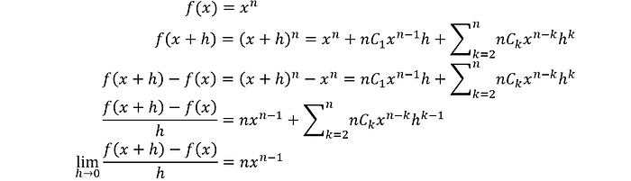
Would this hold true for any n? The binomial coefficients are n(n-1)⋯(n-k+1)/k! for positive n. An extension of this definition for any real number r would be r(r-1)⋯(r-k+1)/k! and the ratio of the (k+1)th coefficient with the kth cofficient is (r-k)/(k+1) which goes to 0 as k goes to infinity. Newton realized that the inifinite series with each term being rCk x^k is the expansion for (1+x)^r for any real r. He did not prove this but verified that the expansion for (1+x)^0.5 when multiplied with itself provides (1+x). It is easy to see that for |x|<1, this series converges since the ratio of (k+1) coefficient to kth coefficient goes to 0 as k becomes large. The proof for the power series expansion is shown below.

Assuming that for (r-1) power (1+x)^(r-1), we have the infinite series expansion, we see that the rth power (1+x)^r also has the corresponding infinite series expansion. Expanding (x+h)^r is same as expanding (x^r)(1+h/x)^r and this power series expansion can be applied to (1+h/x)^r. Newton used this expansion to show that the derivative for x^r is rx^(r-1) for any r. Note that no r will generate the 1/x term as derivative!
The power series expansion for (1+x)^-1 gives us the alternating series 1-x+x²-x³+… and the function f(x) = (1+x)^-1 is a hyperbola that is shifted by 1 unit. Work done by Fermat (of the famous Fermat's last theorem) and other mathematicians around this time led to the understanding that the area under the parabola from 1 to t is logarithmic in t. Since area under the curve is the integral (a.k.a, the anti-derivative), we can conclude that the integral of 1/x is ln(x) and thus the derivative of ln(x) is 1/x. The power series expansion for ln(1+x) can be found by integrating the power series expansion for (1+x)^(-1).
As we are touching upon all the mathematical drama in 17th century Europe, here is another one. Pierre de Fermat made a note in the margin of his copy of Diophantus's "Arithmetica" that he had discovered a truly marvelous proof that the equation a^n + b^n = c^n has no positive integer solutions for n greater than 2 and that the margin was too narrow to contain it. This came to be known as the Fermat's last theorem and several mathematians (both amateur and professional) has since tried to prove or disprove this seeming simple statement. Only in 1990s, Andrew Wiles used all the advanced mathematics of 20th century to prove this elusive theorem. There is no way Fermat could have had a proof 300 years ago!
For other functions that can be written as product of simpler functions, we can apply the product rule to find their derivative. For functions like y = x^x, we have ln(y) = x ln(x) and we can apply product rule on the right. We then have (1/y)(dy/dx) = 1 + ln(x), giving us dy/dx = (x^x)(1+ln(x)).
Much of the modern notation we use today for calculus is given by Gottfried Wilhelm Leibniz of Germany, who independently developed calculus. The name differential calculus comes from Leibniz while Newton called his version "fluxions". There was a bitter dispute as to who invented calculus first. Newton's supporters accused Leibniz of plagiarism, claiming that he had seen Newton's unpublished work during his visit to London.
Newton was a recluse and did not publish much of his work. Leibniz published his analysis first and his version was popularized in Europe by the leading mathematicians of that time. This credit controversy made Newton even more suspicious and he became quite secretive about his work. While the exact extent of exposure Leibniz had to Newton's work remains a subject of debate, modern historians agree that both developed calculus indepdently. But what a drama over the ideas that had been intutively understood for many centuries.
With infinite series sums, there is the question of convergence. The binomial series for (1+x)^r converges only for |x| < 1. Checking for convergence requires evaluating the ratio of two consequent terms and see if it vanishes at the limit. Sometimes, evaluating ratio of functions at the limit results in indeterminate forms like 0/0 or ∞/∞ or 0×∞. If this happens, then instead of looking at the ratio exactly at the limit, we can look at what happens in the neighborhood of the limit. Say the functions f(x) and g(x) are continous in the interval (a,b). Then there exists a point c between a and b at which the slope of the tangent line at point, which is the df(x)/dx, is same as the line joining points a and b.
This is quite easy to visualize. Say f(x) is a line in the interval (a,b), then every point between (a,b) has the same slope as the line joining (a,b). The other possibilities are the f(x) is convex or concave in the interval (a,b), and then there exists a point c at which the the tangent line has the same slope as the secant line connecting a to b.
Written as an equation, this means (f(b)-f(a))/(b-a) = df/dx. If we now let x = b and let x approach a, as long as f(x) is continous in the interval, we have the average slope to be the same as f′=df/dx.
In case f(x)/g(x) when x goes to a certain limit evaluates to an indeterminate form, we can then approximate the value of f(x) and g(x) in the neighborhood of the limit by replacing them with the first derivative — that is, instead of evaluating f(x)/g(x) at some limit of x, we evaluate f′/g′ at that limit. This technique is known as the l'Hôpital's rule, named after the french mathematician Guillaume de l'Hôpital who hired Johann Bernoulli of the renowned Bernoulli family, to tutor him in calculus but also to secretly share with him any latest discoveries Johann Bernoulli made in calculus. In exchange for money, Johann agreed, but later on grew to resent the arrangement, and after l'Hôpital's death, Johann Bernoulli made public that he was the true dicoverer of the rule. Lots of drama in calculus.
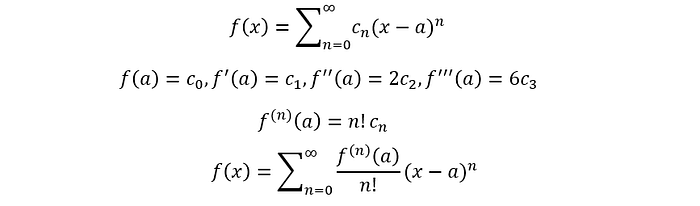
Taylor series extends this idea of approximating a function in the neighbourhood of a point using its derivatives. Let f(x) = ∑c[n](x-a)^n be the power series expansion of f(x) in the neighborhood of x=a. The coefficient c[n] can be found by differentiating f(x) n times and evaluating the result at x=a. All other terms except the (x-a)^n term of f(x) will become zero at x=a, and c[n] is the nth derivative of f(x) at x=a scaled by the n! that naturally arises due to x^n being differentiated n times.
That, my dear reader, is the story of 2000 years of ingeneous ideas. Ideas that gave us a way to compute pi to any precision, formulas to compute trignometric functions with arbitrary accuracy, led to the formalization of calculus and the elegant power series expansion using derivatives. I hope this narrative was as enjoyable as any other story you have encountered, since the characters here are real life legends without whom our understanding of the world would be far poorer.