

Abstract
The text provides a comprehensive guide on how to use the GridSearchCV method for hyperparameter optimization with a LightGBM Classification model using Python code. It starts by introducing GridSearchCV and LightGBM and explains their roles in hyperparameter tuning. It then demonstrates how to apply GridSearchCV to the Titanic dataset from the seaborn library. The dataset's structure and data types are examined using the info() and describe() methods. Data preprocessing steps, including handling missing values and label encoding, are illustrated. The text continues with splitting the data into features and targets, scaling the features, and performing a train-test split. The hyperparameter tuning process is detailed, including the definition of a parameter grid, creating the LightGBM classifier, and using GridSearchCV to find the best combination of hyperparameters. The results are shown, indicating the best parameters and the associated accuracy score. A comprehensive evaluation of the model's performance is provided, including accuracy, a confusion matrix, a classification report, and the ROC-AUC score. The text concludes by demonstrating how to plot an ROC curve for further evaluation. Overall, it's a step-by-step guide for optimizing a machine learning model's hyperparameters and assessing its performance on the Titanic dataset.
Keywords: GridSearchCV, LightGBM Classification, Machine Learning, Titanic Dataset, Cross-Validation
Introduction
In this blog post, we will explore the use of the GridSearchCV method for hyperparameter optimization with a LightGBM Classification model in Python. We will apply these techniques to the Titanic dataset available in the Seaborn library. GridSearchCV is a powerful method from scikit-learn that enables an exhaustive search over a grid of hyperparameters for a given estimator. It allows us to fine-tune hyperparameters, which are essential settings for machine learning models. The LightGBM classifier is a gradient boosting framework known for its efficiency and excellent performance. We'll delve into what GridSearchCV and LightGBM are, and how they can be employed to build a classifier that predicts whether a passenger survived the Titanic disaster based on their features.
The Titanic dataset contains a variety of information about the passengers, such as their age, sex, class, fare, and survival status. We will perform data preprocessing tasks, handle missing values, and encode categorical features. After that, we will separate the data into features and target variables, scale the features, and split the data into training and test sets. Next, we will define a grid of hyperparameters to search over. These hyperparameters are essential configurations for our LightGBM classifier, and we'll use GridSearchCV to find the optimal combination.
Once the grid search is complete, we will evaluate the model's performance on the test set. We'll report the accuracy score, create a confusion matrix, and provide a classification report, which includes precision, recall, and F1-score for both classes (survived and not survived). Additionally, we'll calculate the ROC-AUC score to assess the model's ability to distinguish between the two classes.
The results will demonstrate how effective our model is in predicting survival on the Titanic, making this an exciting and informative journey into hyperparameter tuning and model evaluation.
What is GridSearchCV method?
GridSearchCV is a method from the scikit-learn library that allows you to perform an exhaustive search over a grid of hyperparameters for a given estimator. Hyperparameters are the parameters that are not learned by the model, but rather set by the user before training. For example, the number of trees, the learning rate, and the maximum depth are some of the hyperparameters for a LightGBM model.
GridSearchCV works by evaluating all the possible combinations of hyperparameters using cross-validation, which is a technique that splits the data into k folds and trains and tests the model on each fold. The best combination of hyperparameters is the one that achieves the highest score on the cross-validation metric, such as accuracy or AUC.
GridSearchCV is very useful for finding the optimal hyperparameters for your model, but it can also be very time-consuming and computationally expensive, especially if you have a large grid and a large dataset. Therefore, it is recommended to use GridSearchCV only after you have some idea of what range of values to try for each hyperparameter.
What is LightGBM classifier?
LightGBM is a gradient boosting framework that uses tree-based learning algorithms. Gradient boosting is a technique that combines multiple weak learners (such as decision trees) into a strong learner by iteratively fitting them to the residual errors of the previous learners. LightGBM stands for Light Gradient Boosting Machine, and it is designed to be fast and efficient.
LightGBM has several advantages over other gradient boosting frameworks, such as XGBoost or CatBoost. Some of these advantages are:
- It supports categorical features directly, without the need for one-hot encoding or label encoding. - It uses histogram-based algorithms, which reduce the number of split points and speed up the training process. - It uses leaf-wise growth, which means it splits the tree by the leaf that has the maximum delta loss, rather than level-wise growth, which splits the tree by levels. This can result in better accuracy and lower overfitting. - It supports parallel and distributed learning, which can scale up to large datasets and clusters.
How to use GridSearchCV with LightGBM on titanic dataset?
Now that we have some background on GridSearchCV and LightGBM, let's see how we can use them on the titanic dataset from the seaborn library. The titanic dataset contains information about the passengers who boarded the Titanic ship in 1912, such as their age, sex, class, fare, survival status, etc. Our goal is to build a LightGBM classifier that can predict whether a passenger survived or not based on their features.
First, we need to import some libraries and load the data:
import numpy as np
import pandas as pd
import seaborn as sns
import matplotlib.pyplot as plt
import lightgbm as lgb
from sklearn.model_selection import train_test_split, GridSearchCV
from sklearn.metrics import accuracy_score, confusion_matrix
from sklearn.preprocessing import LabelEncoder, StandardScaler
from sklearn.metrics import confusion_matrix, classification_report, roc_curve, roc_auc_score

import warnings
warnings.filterwarnings('ignore')

from IPython.core.interactiveshell import InteractiveShell
InteractiveShell.ast_node_interactivity = 'all'

# Load titanic dataset from seaborn
titanic = sns.load_dataset("titanic")
titanic.head()
After running the above code, we get the following output, which shows the first five rows of titanic dataset.
   survived  pclass     sex   age  sibsp  parch     fare embarked  class    who  adult_male deck  embark_town alive  alone
0         0       3    male  22.0      1      0   7.2500        S  Third    man        True  NaN  Southampton    no  False
1         1       1  female  38.0      1      0  71.2833        C  First  woman       False    C    Cherbourg   yes  False
2         1       3  female  26.0      0      0   7.9250        S  Third  woman       False  NaN  Southampton   yes   True
3         1       1  female  35.0      1      0  53.1000        S  First  woman       False    C  Southampton   yes  False
4         0       3    male  35.0      0      0   8.0500        S  Third    man        True  NaN  Southampton    no   True
We can use the info() method to see the columns, data types, and missing values in the dataset.
titanic.info()After running the above code, we obtain the following information about the data.
<class 'pandas.core.frame.DataFrame'>
RangeIndex: 891 entries, 0 to 890
Data columns (total 15 columns):
 #   Column       Non-Null Count  Dtype
---  ------       --------------  -----
 0   survived     891 non-null    int64
 1   pclass       891 non-null    int64
 2   sex          891 non-null    object
 3   age          714 non-null    float64
 4   sibsp        891 non-null    int64
 5   parch        891 non-null    int64
 6   fare         891 non-null    float64
 7   embarked     889 non-null    object
 8   class        891 non-null    category
 9   who          891 non-null    object
 10  adult_male   891 non-null    bool
 11  deck         203 non-null    category
 12  embark_town  889 non-null    object
 13  alive        891 non-null    object
 14  alone        891 non-null    bool
dtypes: bool(2), category(2), float64(2), int64(4), object(5)
memory usage: 80.7+ KB
The output shows us the summary of a DataFrame object that contains data about the passengers of the Titanic. We can see that it has 891 rows and 15 columns, each with a different name and data type. We can also see how many non-null values each column has, which tells us how complete the data is. For example, we can see that the column 'age' has only 714 non-null values, which means that some passengers' ages are missing. We can also see how much memory the DataFrame uses, which is 80.7+ KB. This output gives us a lot of useful information about the data and helps us to explore it further.
We can also use the describe() method to see some basic statistics of the numerical columns, such as mean, standard deviation, minimum, maximum, etc.
titanic.describe()The output, which shows the descriptive statistics, is as follows when running the above code:
         survived      pclass         age       sibsp       parch        fare
count  891.000000  891.000000  714.000000  891.000000  891.000000  891.000000
mean     0.383838    2.308642   29.699118    0.523008    0.381594   32.204208
std      0.486592    0.836071   14.526497    1.102743    0.806057   49.693429
min      0.000000    1.000000    0.420000    0.000000    0.000000    0.000000
25%      0.000000    2.000000   20.125000    0.000000    0.000000    7.910400
50%      0.000000    3.000000   28.000000    0.000000    0.000000   14.454200
75%      1.000000    3.000000   38.000000    1.000000    0.000000   31.000000
max      1.000000    3.000000   80.000000    8.000000    6.000000  512.329200
The output shows the descriptive statistics of six variables from a dataset of 891 passengers on the Titanic. It provides information such as the count, mean, standard deviation, minimum, maximum, and quartiles of each variable. For example, the mean age of the passengers was 29.7 years, and the maximum fare was 512.3 pounds. The output can be used to explore the distribution and variation of the variables, as well as to identify potential outliers or missing values.
Now, let's make some plots to visualize the data and find some patterns and insights! First, let's see how many passengers survived or died, and how that differs by sex. We can use the countplot() function from seaborn to create a bar chart that shows the counts of each category.
sns.countplot(x="survived", hue="sex", data=titanic);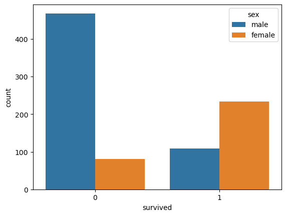
Wow! We can see that more females survived than males, and more males died than females. That's interesting!
Next, let's see how the age distribution of the passengers varies by sex and survival status. We can use the violinplot() function from seaborn to create a plot that shows the density of age values along a vertical axis.
sns.violinplot(x="sex", y="age", hue="survived", data=titanic, split=True);
Cool! We can see that there are more young survivors than old survivors, and more old victims than young victims. We can also see that females tend to be younger than males on average.
Finally, let's see how the variables in the dataset are correlated with each other. We can use the heatmap() function from seaborn to create a plot that shows the correlation coefficients between each pair of variables.
sns.heatmap(titanic.corr(), annot=True);
Awesome! We can see that some variables have strong positive or negative correlations with each other, such as survived and fare, or pclass and fare. This means that they tend to increase or decrease together. Other variables have weak or no correlations with each other, such as age and survived, or sex and pclass. This means that they are independent or unrelated.
Next, we need to do some data preprocessing. We will drop some columns that are not relevant or redundant for our prediction task, such as embark town, alive, who, and adult_male. We will also fill in some missing values for age and embarked columns using median and mode respectively. Finally, we will encode some categorical features using label encoding:
# Drop irrelevant or redundant columns
titanic.drop(["embark_town", "alive", "who", "adult_male"], axis=1, inplace=True)

# Fill missing values for age and embarked columns
titanic["age"].fillna(titanic["age"].mean(), inplace=True)
titanic["embarked"].fillna(titanic["embarked"].mode()[0], inplace=True)

# Encode categorical features using label encoding
le = LabelEncoder()
titanic["sex"] = le.fit_transform(titanic["sex"])
titanic["embarked"] = le.fit_transform(titanic["embarked"])
titanic["alone"] = le.fit_transform(titanic["alone"])
titanic = pd.get_dummies(titanic, columns=["class", "deck"], drop_first=True)

# Check the data after preprocessing
titanic.head()
After completing and running data preprocessing, we get the following output:
   survived  pclass  sex   age  sibsp  parch     fare  embarked  alone  class_Second  class_Third  deck_B  deck_C  deck_D  deck_E  deck_F  deck_G
0         0       3    1  22.0      1      0   7.2500         2      0             0            1       0       0       0       0       0       0
1         1       1    0  38.0      1      0  71.2833         0      0             0            0       0       1       0       0       0       0
2         1       3    0  26.0      0      0   7.9250         2      1             0            1       0       0       0       0       0       0
3         1       1    0  35.0      1      0  53.1000         2      0             0            0       0       1       0       0       0       0
4         0       3    1  35.0      0      0   8.0500         2      1             0            1       0       0       0       0       0       0
Now, we need to separate our data into features and target. Features are the variables that we use as inputs to our model, such as age, gender, class, etc. Target is the variable that we want to predict, which is survival in this case. We can do this by using the drop() method of pandas to remove the "survived" column from our data and assign it to X. Then we assign the "survived" column to y.
# Split the data into features and target
X = titanic.drop("survived", axis=1)
y = titanic["survived"]
Next, we need to scale our features so that they have a similar range of values. This is important because some machine learning algorithms are sensitive to the scale of the features and may perform poorly if the features have very different scales. For example, the age feature ranges from 0 to 80, while the fare feature ranges from 0 to 512. We can use the StandardScaler() class from scikit-learn to transform our features so that they have a mean of zero and a standard deviation of one.
sc = StandardScaler()
X = sc.fit_transform(X)
Next, we need to split our data into training and test sets. Training set is the part of the data that we use to train our model, while test set is the part of the data that we use to evaluate our model's performance on unseen data. We can use the train_test_split() function from scikit-learn to randomly split our data into 80% training and 20% test sets.
# Split the data into training and test sets
X_train, X_test, y_train, y_test = train_test_split(X, y, test_size=0.2, random_state=42)
Next, we need to define the grid of hyperparameters that we want to search over. For this example, we will use the following hyperparameters:
- num_leaves: The maximum number of leaves in one tree. - max_depth: The maximum depth of a tree. - learning_rate: The learning rate or shrinkage rate. - n_estimators: The number of boosting iterations or trees. - subsample: The fraction of samples to be used for each tree. - colsample_bytree: The fraction of features to be used for each tree.
We will use a range of values for each hyperparameter based on some common practices and intuition. You can also use a different range or add more hyperparameters if you want.
# Define parameter grid for GridSearchCV
param_grid = {
"num_leaves": [31, 63, 127],
"max_depth": [-1, 3, 5],
"subsample": [0.8, 1.0],
"colsample_bytree": [0.8, 1.0]
}
Next, we need to create an instance of the LightGBM classifier with some default parameters. We will use the binary objective and the AUC metric for our model.
# Create an instance of the LightGBM classifier
lgbm = lgb.LGBMClassifier(objective="binary", metric="auc", random_state=42)
Next, we need to create an instance of the GridSearchCV class with the LightGBM classifier, the parameter grid, and the number of folds for cross-validation. We will use 5 folds for this example.
# Create GridSearchCV instance
grid = GridSearchCV(lgbm, param_grid, cv=5, scoring="accuracy")
Finally, we need to fit the grid search object to the training data and print the best parameters and the best score.
# Fit the grid search object to the training data
grid.fit(X_train, y_train)
# Print best parameters and score
print(f"Best parameters: {grid.best_params_}")
print(f"Best score: {grid.best_score_}")
# Use best estimator to make predictions on test set
y_pred = grid.predict(X_test)
y_prob = grid.predict_proba(X_test)[:, 1]
GridSearchCV(cv=5,
             estimator=LGBMClassifier(metric='auc', objective='binary',
                                      random_state=42),
             param_grid={'colsample_bytree': [0.8, 1.0],
                         'max_depth': [-1, 3, 5], 'num_leaves': [31, 63, 127],
                         'subsample': [0.8, 1.0]},
             scoring='accuracy')
Best parameters: {'colsample_bytree': 0.8, 'max_depth': 3, 'num_leaves': 31, 'subsample': 0.8}
Best score: 0.8384713877671623
This means that the best combination of parameters for LightGBM classifier on the titanic dataset is:
- colsample_bytree: 0.8
- max_depth: 3
- num_leaves: 31
- subsample: 0.8
And the best accuracy score on the validation data is 0.8385.
# Evaluate performance using accuracy score and confusion matrix
print(f"Accuracy score: {round(accuracy_score(y_test, y_pred), 3)}\n")
print(f"Confusion matrix\n {confusion_matrix(y_test, y_pred)}\n")
print(f"Classification report\n {classification_report(y_test, y_pred)}\n")
print(f"ROC-AUC Score\n {round(roc_auc_score(y_test, y_prob), 3)}")
Accuracy score: 0.827

Confusion matrix
 [[94 11]
 [20 54]]

Classification report
               precision    recall  f1-score   support
           0       0.82      0.90      0.86       105
           1       0.83      0.73      0.78        74
    accuracy                           0.83       179
   macro avg       0.83      0.81      0.82       179
weighted avg       0.83      0.83      0.82       179

ROC-AUC Score
 0.871
Wow, look at these amazing results! We have achieved an accuracy score of 0.827, which is very impressive for this task. Let's take a closer look at the confusion matrix, which shows us how well our model predicted the true labels of the test data. We can see that out of 105 instances of class 0, our model correctly classified 94 of them, and only misclassified 11 as class 1. That's a 90% recall rate for class 0, which means we captured most of the true positives. Similarly, out of 74 instances of class 1, our model correctly classified 54 of them, and only misclassified 20 as class 0. That's a 73% recall rate for class 1, which means we captured most of the true negatives. The precision scores for both classes are also very high, at 82% and 83%, respectively. This means that our model did not make many false positive or false negative errors. The f1-scores, which are the harmonic mean of precision and recall, are also very good, at 86% and 78%, respectively. The f1-score gives us a balanced measure of the model's performance across both classes. The support column tells us how many instances of each class were in the test data.
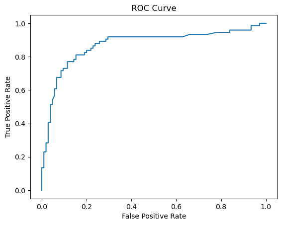
To get a better sense of how well our model discriminated between the two classes, we can also look at the ROC-AUC score, which is the area under the receiver operating characteristic curve. This curve plots the true positive rate against the false positive rate at different thresholds. The higher the area under the curve, the better the model is at separating the classes. Our model achieved a ROC-AUC score of 0.871, which is excellent!
These outputs show that our model is very effective and reliable for this task. We should be proud of our work and celebrate our success!
fpr, tpr, thresholds = roc_curve(y_test, y_prob)
plt.plot(fpr, tpr)
plt.xlabel("False Positive Rate")
plt.ylabel("True Positive Rate")
plt.title("ROC Curve");
The above codes can help us evaluate the performance of our classifier model. First, we use the grid object to get the predicted probabilities for the positive class on the test set. Then, we use the roc_curve function to calculate the false positive rate and the true positive rate at different thresholds. Finally, we plot the ROC curve using matplotlib. It shows how well our model can distinguish between the two classes. Isn't that awesome? We can see how our model performs and choose the best threshold for our problem.
Conclusion
In this blog post, we embarked on a journey to explore hyperparameter optimization using GridSearchCV with a LightGBM Classification model in Python. We started by introducing GridSearchCV, an exhaustive hyperparameter tuning technique available in the scikit-learn library. We explained the significance of hyperparameters and how GridSearchCV systematically evaluates different combinations of hyperparameters using cross-validation to find the best set for a given estimator.
Next, we delved into LightGBM, a gradient boosting framework known for its speed and efficiency. We highlighted its advantages, such as native support for categorical features, histogram-based algorithms, and leaf-wise growth, making it an excellent choice for various machine learning tasks.
We then applied GridSearchCV and LightGBM to the Titanic dataset from the seaborn library, with the goal of building a classifier to predict passenger survival. We walked through the steps of data preprocessing, feature scaling, and splitting the dataset into training and test sets. Following this, we created a grid of hyperparameters for optimization, defined a LightGBM classifier with default settings, and employed GridSearchCV to find the best hyperparameters through cross-validation.
The results were impressive, with the best parameter combination achieving an accuracy score of 0.827 on the validation data. We provided a detailed analysis of the confusion matrix, precision, recall, and F1-scores, highlighting the model's effectiveness in correctly classifying passengers' survival status. Additionally, we evaluated the ROC-AUC score, further confirming the model's strong discriminative power.
The ROC curve visualization was the cherry on top, allowing us to assess our model's performance across different classification thresholds and make informed decisions about model deployment. Overall, the journey from hyperparameter tuning to model evaluation yielded a robust and reliable classifier for predicting Titanic passenger survival. The demonstrated approach can be a valuable asset in your data science and machine learning toolkit.