

In this article, we will look at seven popular methods for subset selection and shrinkage in linear regression. After an introduction to the topic justifying the need for such methods, we will look at each approach one by one, covering both mathematical properties and a Python application.
This article is based on a chapter from the excellent Hastie, T., Tibshirani, R., & Friedman, J. H. (2009). The elements of statistical learning: data mining, inference, and prediction. 2nd ed. New York: Springer. Some technical details might be paraphrased or quoted directly.

Why shrink or subset and what does this mean?
In the linear regression context, subsetting means choosing a subset from available variables to include in the model, thus reducing its dimensionality. Shrinkage, on the other hand, means reducing the size of the coefficient estimates (shrinking them towards zero). Note that if a coefficient gets shrunk to exactly zero, the corresponding variable drops out of the model. Consequently, such a case can also be seen as a kind of subsetting.
Shrinkage and selection aim at improving upon the simple linear regression. There are two main reasons why it could need improvement:
- Prediction accuracy: Linear regression estimates tend to have low bias and high variance. Reducing model complexity (the number of parameters that need to be estimated) results in reducing the variance at the cost of introducing more bias. If we could find the sweet spot where the total error, so the error resulting from bias plus the one from variance, is minimized, we can improve the model's predictions.
- Model's interpretability: With too many predictors it is hard for a human to grasp all the relations between the variables. In some cases we would be willing to determine a small subset of variables with the strongest impact, thus sacrificing some details in order to get the big picture.
Setup & Data Load
Before jumping straight to the methods themselves, let us first look at the data set we will be analyzing. It comes from a study by Stamey et al. (1989) who investigated the impact of different clinical measurements on the level of prostate-specific antigen (PSA). The task is to identify the risk factors for prostate cancer, based on a set if clinical and demographic variables. The data, together with some descriptions of the variables, can be found on the website of Hastie's et al. "The elements of statistical learning" textbook, in the Data section.
We will start by importing the modules used throughout this article, loading the data, and splitting it into training and testing sets, keeping the targets and the features separately. We will then discuss each of the shrinkage and selection methods, fit it to the training data, and use the test set to check how well can it predict the PSA levels on new data.
Linear Regression
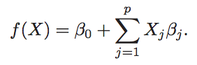
Let us start with the simple linear regression, which will constitute our benchmark. It models the target variable, y, as a linear combination of p predictors, or features, X:
This model has p + 2 parameters that have to be estimated from the training data:
- The p feature β-coefficients, one per variable, denoting their impacts on the target;
- One intercept parameter, denoted as β0 above, which is the prediction in case all Xs are zero. It is not necessary to include it in the model, and indeed in some cases, it should be dropped (e.g. if one wants to include a full set of dummies denoting levels of a categorical variable) but in general it gives the model more flexibility, as you will see in the next paragraph;
- One variance parameter of the Gaussian error term.
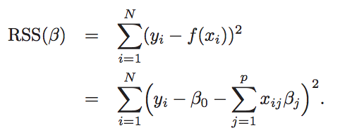
These parameters are typically estimated using Ordinary Least Square (OLS). OLS minimizes the sum of squared residuals, given by
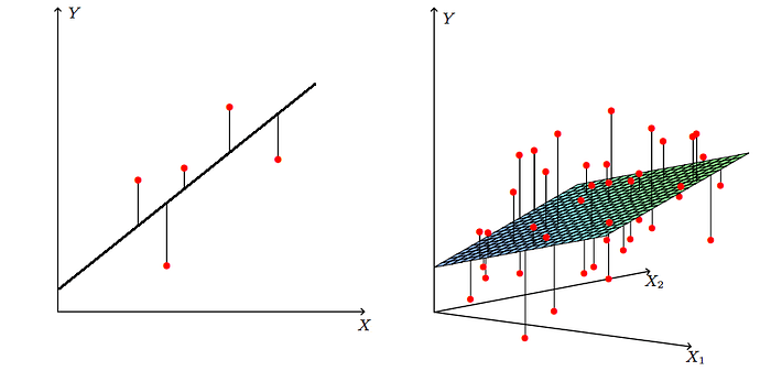
It is helpful to think about this minimization criterion graphically. With only one predictor X, we are in a 2D space, formed by this predictor and the target. In this setting, the model fits such a line in the X-Y space that is the closest to all data points, with the proximity measured as the sum of squared vertical distances of all data points — see the left panel below. If there are two predictors, X1 and X2, space grows to 3D and now the model fits a plane that is closest to all points in the 3D space — see the right panel below. With more than two features, the plane becomes the somewhat abstract hyperplane, but the idea is still the same. These visualizations also help to see how the intercept gives the model more flexibility: if it is included, it allows the line or plane to not cross the space's origin.
The minimization problem described above turns out to have an analytical solution, and the β-parameters can be calculated as
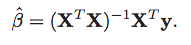
Including a column of ones in the X matrix allows us to express the intercept part of the β-hat vector in the formula above. The "hat" above the "β" denotes that it is an estimated value, based on the training data.
The Bias-Variance trade-off
In statistics, there are two critical characteristics of estimators to be considered: the bias and the variance. The bias is the difference between the true population parameter and the expected estimator. It measures the inaccuracy of the estimates. The variance, on the other hand, measures the spread between them.
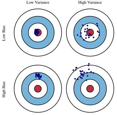
Clearly, both bias and variance can harm the model's predictive performance if they are too large. The linear regression, however, tends to suffer from variance, while having a low bias. This is especially the case if there are many predictive features in the model or if they are highly correlated with each other. This is where subsetting and regularization come to rescue. They allow reducing the variance at the cost of introducing some bias, ultimately reducing the total error of the model.
Before discussing these methods in detail, let us fit a linear regression to out prostate data and check its out-of-sample Mean Prediction Error (MAE).
Best Subset Regression
A straightforward approach to choosing a subset of variables for linear regression is to try all possible combinations and pick one that minimizes some criterion. This is what Best Subset Regression aims for. For every k ∈ {1, 2, …, p}, where p is the total number of available features, it picks the subset of size k that gives the smallest residual sum of squares. However, the sum of squares cannot be used as a criterion to determine k itself, as it is necessarily decreasing with k: the more variables are included in the model, the smaller are its residuals. This does not guarantee better predictive performance though. That's why another criterion should be used to select the final model. For models focused on prediction, a (possibly cross-validated) error on test data is a common choice.
As Best Subset Regression is not implemented in any Python package, we have to loop over k and all subsets of size k manually. The following chunk of code does the job.
Ridge Regression
One drawback of Best Subset Regression is that it does not tell us anything about the impact of the variables that are excluded from the model on the response variable. Ridge Regression provides an alternative to this hard selection of variables that splits them into included in and excluded from the model. Instead, it penalizes the coefficients to shrink them towards zero. Not exactly zero, as that would mean exclusion from the model, but in the direction of zero, which can be viewed as decreasing model's complexity in a continuous way, while keeping all variables in the model.
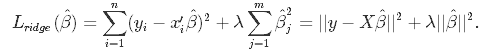
In Ridge Regression, the Linear Regression loss function is augmented in such a way to not only minimize the sum of squared residuals but also to penalize the size of parameter estimates:
Solving this minimization problem results in an analytical formula for the βs:
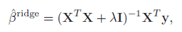
where I denotes an identity matrix. The penalty term λ is a hyperparameter to be chosen: the larger its value, the more are the coefficients shrunk towards zero. One can see from the formula above that as λ goes to zero, the additive penalty vanishes, and β-ridge becomes the same as β-OLS from linear regression. On the other hand, as λ grows to infinity, β-ridge approaches zero: with high enough penalty, coefficients can be shrunk arbitrarily close to zero.
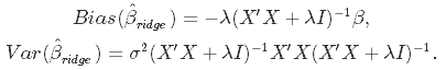
But does this shrinkage really result in reducing the variance of the model at the cost of introducing some bias as promised? Yes, it does, which is clear from the formulae for ridge regression estimates' bias and variance: as λ increases, so does the bias, while the variance goes down!
Now, how to choose the best value for λ? Run cross-validation trying a set of different values and pick one that minimizes cross-validated error on test data. Luckily, Python's scikit-learn can do this for us.
LASSO
Lasso, or Least Absolute Shrinkage and Selection Operator, is very similar in spirit to Ridge Regression. It also adds a penalty for non-zero coefficients to the loss function, but unlike Ridge Regression which penalizes the sum of squared coefficients (the so-called L2 penalty), LASSO penalizes the sum of their absolute values (L1 penalty). As a result, for high values of λ, many coefficients are exactly zeroed under LASSO, which is never the case in Ridge Regression.
Another important difference between them is how they tackle the issue of multicollinearity between the features. In Ridge Regression, the coefficients of correlated variables tend to be similar, while in LASSO one of them is usually zeroed and the other is assigned the entire impact. Because of this, Ridge Regression is expected to work better if there are many large parameters of about the same value, i.e. when most predictors truly impact the response. LASSO, on the other hand, is expected to come on top when there are a small number of significant parameters and the others are close to zero, i.e. when only a few predictors actually influence the response.
In practice, however, one doesn't know the true values of the parameters. So, the choice between Ridge Regression and LASSO can be based on an out-of-sample prediction error. Another option is to combine these two approaches in one — see the next section!
LASSO's loss function looks as follows:
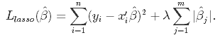
Unlike in Ridge Regression, this minimization problem cannot be solved analytically. Fortunately, there are numerical algorithms able to deal with it.
Elastic Net
Elastic Net first emerged as a result of critique on LASSO, whose variable selection can be too dependent on data and thus unstable. Its solution is to combine the penalties of Ridge Regression and LASSO to get the best of both worlds. Elastic Net aims at minimizing the loss function that includes both the L1 and L2 penalties:
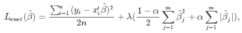
where α is the mixing parameter between Ridge Regression (when it is zero) and LASSO (when it is one). The best α can be chosen with scikit-learn's cross-validation-based hyperparameter tuning.
Least Angle Regression
So far we have discussed one subsetting method, Best Subset Regression, and three shrinkage methods: Ridge Regression, LASSO, and their combination, Elastic Net. This section is devoted to an approach located somewhere in between subsetting and shrinking: Least Angle Regression (LAR). This algorithm starts with a null model, with all coefficients equal to zero, and then works iteratively, at each step moving the coefficient of one of the variables towards its least squares value.
More specifically, LAR starts with identifying the variable most correlated with the response. Then it moves the coefficient of this variable continuously toward its least squares value, thus decreasing its correlation with the evolving residual. As soon as another variable "catches up" in terms of correlation with the residual, the process is paused. The second variable then joins the active set, i.e. the set of variables with non-zero coefficients, and their coefficients are moved together in a way that keeps their correlations tied and decreasing. This process continues until all the variables are in the model and ends at the full least-squares fit. The name "Least Angle Regression" comes from the geometrical interpretation of the algorithm in which the new fit direction at a given step makes the smallest angle with each of the features that already have non-zero coefficients.
The code chunk below applies LAR to the prostate data.
Principal Components Regression
We have already discussed methods for choosing variables (subsetting) and decreasing their coefficients (shrinkage). The last two methods explained in this article take a slightly different approach: they squeeze the input space of the original features into a lower-dimensional space. Mainly, they use X to create a small set of new features Z that are linear combinations of X and then use those in regression models.
The first of these two methods is Principal Components Regression. It applies Principal Components Analysis, a method allowing to obtain a set of new features, uncorrelated with each other, and having high variance (so that they can explain the variance of the target), and then uses them as features in simple linear regression. This makes it similar to Ridge Regression, as both of them operate on the principal components space of the original features (for PCA-based derivation of Ridge Regression see [1] in Sources at the bottom of this article). The difference is that PCR discards the components with the least informative power, while Ridge Regression simply shrinks them stronger.
The number of components to retain can be viewed as a hyperparameter and tuned via cross-validation, as is the case in the code chunk below.
Partial Least Squares
The final method discussed in this article is Partial Least Squares (PLS). Similarly to Principal Components Regression, it also uses a small set of linear combinations of the original features. The difference lies in how these combinations are constructed. While Principal Components Regression uses only X themselves to create the derived features Z, Partial Least Squares additionally uses the target y. Hence, while constructing Z, PLS seeks directions that have high variance (as these can explain variance in the target) and high correlation with the target. This stays in contrast to the principal components approach, which focuses on high variance only.
Under the hood of the algorithm, the first of the new features, z1, is created as a linear combination of all features X, where each of the Xs is weighted by its inner product with the target y. Then, y is regressed on z1 giving PLS β-coefficients. Finally, all X are orthogonalized with respect to z1. Then the process starts anew for z2 and goes on until the desired numbers of components in Z are obtained. This number, as usual, can be chosen via cross-validation.
It can be shown that although PLS shrinks the low-variance components in Z as desired, it can sometimes inflate the high-variance ones, which might lead to higher prediction errors in some cases. This seems to be the case for our prostate data: PLS performs the worst among all the discussed methods.
Recap & Conclusions
With many, possibly correlated features, linear models fail in terms of prediction accuracy and model's interpretability due to large variance of the model's parameters. This can be alleviated by reducing the variance, which can only happen at the cost of introducing some bias. Yet, finding the best bias-variance trade-off can optimize the model's performance.
Two broad classes of approaches allowing to achieve this are subsetting and shrinkage. The former selects a subset of variables, while the latter shrinks the coefficients of the model towards zero. Both approaches result in a reduction of the model's complexity, which leads to the desired decrease in parameters' variance.
This article discussed a couple of subsetting and shrinkage methods:
- Best Subset Regression iterates over all possible feature combination to select the best one;
- Ridge Regression penalizes the squared coefficient values (L2 penalty) enforcing them to be small;
- LASSO penalizes the absolute values of the coefficients (L1 penalty) which can force some of them to be exactly zero;
- Elastic Net combines the L1 and L2 penalties, enjoying the best of Ridge and Lasso;
- Least Angle Regression fits in between subsetting and shrinkage: it works iteratively, adding "some part" of one of the features at each step;
- Principal Components Regression performs PCA to squeeze the original features into a small subset of new features and then uses those as predictors;
- Partial Least Squares also summarizes original features into a smaller subset of new ones, but unlike PCR, it also makes use of the targets to construct them.
As you will see from the applications to the prostate data if you run the code chunks above, most of these methods perform similarly in terms of prediction accuracy. The first 5 methods' errors range between 0.467 and 0.517, beating least squares' error of 0.523. The last two, PCR and PLS, perform worse, possibly due to the fact that there are not that many features in the data, hence gains from dimensionality reduction are limited.
Thanks for reading! I hope you have learned something useful that will benefit your projects 🚀
If you liked this post, try one of my other articles. Can't choose? Pick one of these:
Sources
- Hastie, T., Tibshirani, R., & Friedman, J. H. (2009). The elements of statistical learning: data mining, inference, and prediction. 2nd ed. New York: Springer.
- https://www.datacamp.com/community/tutorials/tutorial-ridge-lasso-elastic-net