In machine learning, the concept of error is often used as a measure of how well models have learned from the data they were provided. In general, the total error of any given model can be broken down into the sum of three partitions: bias, variance, and noise. In this article, we will explore these quantities in a conceptual framework to assess the quality of our models.

Before diving into error, recall the key objective for a model — to "learn" a simplified understanding of data to make reliable predictions. We define two ends of this learning spectrum: generalization and memorization. An effective model is one that leverages learned generalizations of the training data to accurately make predictions on testing data. On the other hand, a model that has memorized the data fails to generalize beyond the training data, as it has fit itself to perfectly model only those data. As a result, model performance is limited as it is useless outside of the training data. Error is intimately linked to this concept and will be a focal point of our discussion.

Model Bias

Intuitively, bias represents the error from using a model that makes fundamentally different assumptions than the true patterns present in the data. More specifically, it is present when our model makes overly-simplistic assumptions about the data that lead to systematic errors in predictions. For example, assume we attempt to fit a linear model to data that follow a quadratic trend.

No matter how much data it is presented, the model will consistently miss the true relationship since it lacks the flexibility of higher-order parameters. In other words, there exists no linear function that can accurately fit a quadratic function.

This leads to our model underfitting the data. Models with high bias are unable to capture nuances of the data which leads to poor performance both on the training set and when making predictions on new, unseen data. In other words, a model with high bias makes weak generalizations of the training data. Therefore, bias and model simplicity are directly related to one another; the simpler the model, the higher its bias.

Model Variance

We can interpret variance as a measure of model stability — the degree to which the parameters of a model change when trained on random samples of the data. In the case of a linear model, variance would be the fluctuations in values for the y-intercept and slope for different samples from the original data.

It is easiest to understand variance with a visual example. Recall the quadratic data from earlier (Fig. 1). We will fit 1st, 2nd, 5th, and 10th-degree polynomial models to 10 random samples of size 10 from these data:

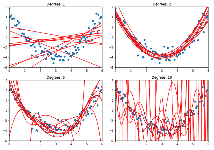
We can observe that the variation between models of the same degree increases with the degree of the model. Visually, this makes sense, as n-degree polynomial functions have n + 1 parameters to fit onto the data. As a result, the models increase in complexity and are able to capture intricate patterns and nuances present in the data. However, this increased flexibility makes models more prone to overfitting, essentially fitting the training data too well to the point that it offers no meaningful simplification of the data and cannot make good predictions on data outside of the training set. In other words, a model with high variance is memorizing the training set rather than learning a transferrable understanding of it. Therefore, variance and model complexity are directly related to one another; the more complex the model, the higher its variance.

Noise

Noise is more broadly defined as the random and unwanted fluctuations that can obscure the data generating process. Just as static can distort or mask the music or speech on a radio, noise in data can distort or hide the real patterns or information we're trying to understand. It comes from various sources, such as measurement errors, environmental factors, or inherent randomness in the system being observed. Unfortunately, this makes noise an irreducible error, as it will always be present so long as data are collected. The best way to handle noise is to be aware of the limitations of the data themselves and incorporate the awareness into any analyses done with the model.

The Trade-off

Given the definitions of the three types of error, it is reasonable to claim that a good model is one that minimizes all three quantities. Since noise is irreducible, we can instead focus on minimizing bias and variance. Reducing bias involves minimizing the error from simplistic assumptions, often requiring increasing model complexity. Conversely, reducing variance involves improving generalization to new data, often requiring a simplification of the model. Therein lies the dilemma — it is impossible to simultaneously decrease both the bias and variance of a model. To solve this problem, we must settle for a model that achieves the minimum combination of these quantities. It is reasonable to draw parallels between this trade-off and that of under- and overfitting data since the bias vs. variance trade-off is a formal statement of balancing model fit. We can represent this visually with bias and variance as functions of model complexity:

The degree of the optimal model would be the complexity value at which the combination of variance and bias are minimum. This would be where the model has low enough bias to avoid underfitting and low enough variance to avoid overfitting. In the case of the quadratic data, we would expect this point to indicate that the optimal model is a second-degree polynomial. It is important to note that bias and variance cannot be computed in practice, because they depend on knowledge of the underlying function that produced the data. Thus, the notions of bias and variance serve more as a conceptual tool that we can utilize to guide model development. In future articles, we will explore strategies to diagnose and address this trade-off, including techniques like cross-validation, regularization, and ensemble methods. Stay tuned!