
If you take a look at the industrial data you would see that in many places we are still using classical Machine Learning algorithms. There is a good reason to use classical ML and AI algorithms over new Deep learning-based methods in industrial settings; the amount and quality of proprietary data. Most banks still use some variant of XGBoost for tabular data. We have seen crazy progress in Deep Learning models, but there are still many fields where growth has been barely linear. One such field where we have seen limited growth is time series forecasting.
Topics Covered
- Understanding Time Series Data
- Turing Completeness
- Other Challenges And Approaches
- Foundational Models As Zero-Shot Forecasters (Chronos and TimesFM)
- Successor of LSTM: xLSTM
- Conclusion
Understanding Time Series Data
Time series data is one of the most naturally occurring forms of data. From internet usage to smart bands, from weather data to the stock market, everything comes under the umbrella of the Time series.
Time series is similar to predicting the future based on past events for a given number of quantities/attributes.
Time series data exhibit dependencies across time steps, known as autocorrelation. Capturing these dependencies requires models to understand both short-term and long-term relationships within the data.
Capturing long-term dependency is something that most Deep-learning models are not particularly good at. Now some of you might say what about LSTMs and RNNs, and you are right. They are indeed good for time series type of data.
But we should understand that these models are very different than CNNs and Transformers, they are actually Turing Complete and that's why they can handle time series.
Turing Completeness
If you are a Computer science grad, you should definitely understand what Turing Complete means. This forms the theoretical basis of what type of system can solve what type of challenges.
Turing machines are theoretical computers defined by Alan Turing in his highly influential paper titled On Computable Numbers, with an application to the Entscheidungsproblem, published 1936. Turing machines are abstract mathematical constructs that help us describe in a rigorous fashion what we mean by computation.
A Turing machine consists of 2 elements: The computational head and an infinitely long tape. The head operates roughly as a 'read-write' head on a disk drive, and the tape is divided up into an infinitely long set of squares, for which on each square a symbol can be written or erased. The Turing machine recognizes and can write down a finite set of symbols, called the Turing machine's alphabet.
The Turing machine is only 'aware' of one square on the tape at a time — namely, the square the head of the Turing machine is currently on.
On that tape, a Turing Machine can do any of these 4 actions:
- Move the head left by 1 space
- Move the head right by 1 space
- Write a symbol at the head
- Erase a symbol at the head
The machine decides which of these operations to do on any given step through a finite state machine. Different Turing machines have different state machines that define their operation.
This is all fine theory-wise, but how does it relate to our problem of time series?
A model is Turing complete if it can simulate any Turing machine, implying it can compute anything that is computable, given sufficient time and resources.
Since models don't have infinite memory, they need to remember and forget a few things, and this level of control is not that easy with Deep learning models. Most Deep-learning models will remember short-term interactions and are not very good at handling long-term dependencies.
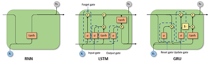
And that's where LSTM and RNNs shine. RNNs have their own limitations, but the LSTM was king in time series for quite some time. We will also see what happened to LSTMs in a bit.
Different types of deep learning architecture exploit different types of symmetries and except LSTM most are not designed for Time series type of data.
Transformers which these days form the backbone of all the major AI models, are not inherently designed for time-related stuff.
If you want to know more about this:
Wikipedia: Turing Completeness
Other Challenges And Approaches
Deep learning models typically require huge amounts of data to train effectively. In many time series applications, especially those with limited historical data, classic methods perform adequately without the need for extensive datasets.
Time series data often exhibit non-stationary behavior, seasonality, and trends. Preparing such data for deep learning can be more challenging compared to classic methods that are inherently designed to handle these characteristics. Another big challenge in Time Series Data is to align two-time series sequences.
Another big challenge is that Deep learning models can easily overfit and are black box in nature. Being able to explain the prediction might be as important as actually predicting in a few cases.
All these reasons combined, we see far fewer Deep learning models in time series compared to image and text modality.
In the past, we tried different models like Temporal Convolutional Networks (TCNs), Transformer-based models, and hybrid approaches combining classic and deep learning methods, but their generalization and accuracy remained questionable.
But now that we have LLMs that have seen enormous amounts of data, practically the entire internet, we can actually have good Transformer-based time series models.
Foundational Models As Zero-Shot Forecasters
LLMs or foundation models as Zero-Shot has various advantages.
- The training set is broad enough, that it should have reasonable performance on unseen data regardless of their granularity, frequencies, sparsity, and perhaps even distribution.
- You don't need to wait until you have enough data to train a model from scratch (eg. ARIMA but might also apply to a global model such as XGBoost).
- When the data starts to come in, you can fine-tune the zero-shot model to your domain (or |other purposes, eg, conformal predictions).
Here are some dataset for training zero-shot forecasters.
Unfortunately, unlike NLP we don't have good datasets for Time Series evaluation.
To solve the data issue, Synthetic data comes in. Generating synthetic data for time series is relatively easier compared to images and videos.
Chronos
"Chronos: Learning the Language of Time Series" is not a single model but it introduces a framework that leverages transformer-based language models for probabilistic time series forecasting.
The core innovation of Chronos is tokenizing continuous time series data into discrete tokens, enabling the application of language modeling techniques.
Tokenization of Time Series:
- Scaling: Each time series is normalized by dividing its values by the mean of their absolute values, ensuring consistency across different scales.
- Quantization: The scaled values are discretized into a fixed number of bins, converting continuous data into a sequence of tokens.
Chronos utilizes the T5 transformer architecture, with model sizes ranging from 20 million to 710 million parameters. The vocabulary size is adjusted to match the number of quantization bins.
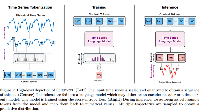
The model is trained using the cross-entropy loss function, treating the forecasting task as a sequence prediction problem. Training data comprises a large collection of publicly available time series datasets, supplemented by synthetic data generated via Gaussian processes to enhance generalization.
By framing time series forecasting as a language modeling problem, Chronos simplifies the forecasting pipeline. Its ability to generalize across diverse datasets without additional training positions it as a versatile tool for various forecasting applications. But as I said time series is a bit different than language prediction. But this is an interesting approach nonetheless.
TimesFM
This is a closed-source model from Google, but this is a completely new architecture designed specifically for time series.
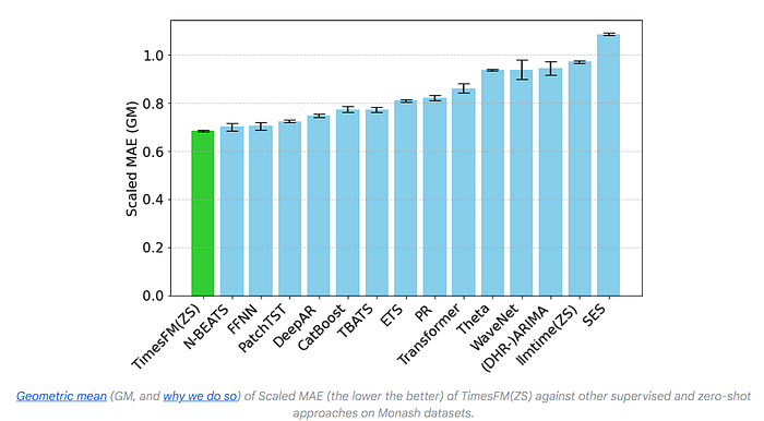
TimesFM is a forecasting model, pre-trained on a large time-series corpus of 100 billion real-world time-points, that displays impressive zero-shot performance on a variety of public benchmarks from different domains and granularities.
Chronos converts continuous time-series values into discrete tokens through normalization and quantization. These tokens are then fed to the transformer layers.
On the other hand, TimesFM uses a different approach. TimesFM treats a patch of time series (a contiguous group of time points) as a token. The patches are processed using an MLP with residual connections before being input to the transformer. It focuses on learning temporal patterns directly from the continuous time-series data without discretization.
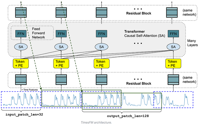
Instead of doing token-by-token prediction, TimesFM is explicitly designed for long-horizon forecasting by using larger output patches, which reduce the number of sequential prediction steps needed, improving both efficiency and accuracy.
But let's go a little deeper, you might still have doubts about TimesFM workings.
Why We Can't Directly Feed Time-Series Patches into Transformers?
Transformers Expect Fixed-Dimensional Inputs:
- Transformers process sequences of tokens, where each token is typically a fixed-length vector.
- Raw time-series patches are matrices (e.g., patch length×features) and vary in size depending on the patch length and feature count. This is incompatible with the fixed-dimensional token input requirement.
Lack of Feature Aggregation:
Without the MLP block, the transformer would treat each individual time point or feature as a separate token. This can lead to:
- Increased computational overhead.
- Loss of meaningful interactions between features within a patch.
Transformer Computation Costs:
- Transformers scale poorly with sequence length (O(n²) for attention mechanisms). Feeding raw time-series patches directly would result in excessive computational costs for long time-series data.
Positional Dependency:
- Raw patches do not inherently carry positional information. Without the MLP block incorporating positional encodings, the transformer would not understand the temporal ordering of data points within the patch.
The MLP block takes a patch of size patch length×features as input. It processes the patch using linear layers to combine and reduce features, applies nonlinear activations to capture higher-order patterns, and employs residual connections for stability and better gradient flow. The output is a fixed-dimensional vector (e.g., hidden size) that serves as a token for the transformer.
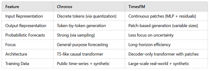
A small table to compare Chronos and TimesFM.
Successor of LSTM: xLSTM
LSTMs have three main limitations:
(i) Inability to revise storage decisions: LSTM struggles to revise a stored value when a more similar vector is found, while our new xLSTM remediates this limitation by exponential gating. Basically, if something is forgotten in the previous state somehow, we can't retrieve it, because the memory in LSTM is preserved in some cell state, not the actual information.
(ii) Limited storage capacities: Information must be compressed into scalar cell states. This limitation is exemplified via Rare Token Prediction. LSTM performs worse on rare tokens because of its limited storage capacities. The new xLSTM solves this problem by a matrix memory.
(iii) Lack of parallelizability due to memory mixing: the hidden-hidden connections between hidden states from one time step to the next, which enforce sequential processing. This is the biggest problem of LSTM as to not being able to use the GPU parallelizability to its full extent.
To overcome the LSTM limitations, Extended Long Short-Term Memory (xLSTM) introduces two main modifications. These modifications — exponential gating and novel memory structures — enrich the LSTM family by two members: (i) the new sLSTM with a scalar memory, a scalar update, and memory mixing, and (ii) the new mLSTM with a matrix memory and a covariance (outer product) update rule, which is fully parallelizable.
Both sLSTM and mLSTM enhance the LSTM through exponential gating. To enable parallelization, the mLSTM abandons memory mixing, i.e., the hidden-hidden recurrent connections. Both mLSTM and sLSTM can be extended to multiple memory cells, where sLSTM features memory mixing across cells. Further, the sLSTM can have multiple heads without memory mixing across the heads, but only memory mixing across cells within each head. This introduction of heads for sLSTM together with exponential gating establishes a new way of memory mixing. For mLSTM multiple heads and multiple cells are equivalent.
This new variant of LSTM has shown significant potential once again in time series forecasting, and even beating the foundational model-based Time series models.
Read full article on xLSTM here:
Conclusion
Regarding foundational time series models, we are still in the early stage of research. We are yet to explore the effect of fine-tuning, creating better evaluation benchmarks, and much more. Synthetic data is also something that needs to be exploited much more. With this, we mark the end of our blog on Time Series Forecasting.
Thank you for reading! If you enjoyed this article and want more insights on AI, consider subscribing to my newsletter. Get exclusive content, updates, and resources directly to your inbox: https://medium.com/aiguys/newsletter
Writing such articles requires considerable effort and time. I would highly appreciate your support through claps and shares. Your engagement motivates me to write more beyond the hype on SOTA AI topics with the utmost clarity and simplicity.
Don't forget to follow me on 𝕏.