Discretization, also known as binning, is a data preprocessing technique used in machine learning to transform continuous features into discrete ones. This transformation helps to handle outliers, reduce noise, and improve model performance. In this article, we'll explore different binning techniques, their definitions, formulas, advantages, and how to implement them using Python.

Unsupervised Binning

1. Equal Width Binning (Uniform)

Definition: Equal width binning divides the data range into intervals of equal size.

Formula:

Explanation: The data is divided into NNN intervals of equal width. Each bin has the same range, but the number of data points in each bin can vary.

Advantages:

• Simple to implement.
• Handles outliers by putting them in separate bins.
• No change in the spread of data.

2. Equal Frequency Binning (Quantile)

Definition: Equal frequency binning divides the data into intervals that contain approximately the same number of data points.

Formula: There is no explicit formula for this method, as it relies on sorting the data and dividing it into bins with equal counts.

Explanation: The data is sorted, and each bin is assigned an equal number of data points. This method ensures that each bin has the same number of observations.

Advantages:

• Handles outliers by distributing them evenly.
• Ensures a uniform spread of data.

3. K-Means Binning

Definition: K-means binning clusters the data using the k-means algorithm and then assigns each cluster to a bin.

Explanation: The k-means algorithm finds kkk centroids in the data. Each data point is assigned to the nearest centroid, and the centroids represent the bin values.

Advantages:

• Useful when data is clustered.
• Bins reflect natural groupings in the data.

Custom Binning

Equal Width Binning (Uniform)

Definition: Similar to unsupervised equal width binning, but the number of bins and their widths are chosen based on domain knowledge or specific requirements.

Code Implementation

Let's implement these binning techniques using a dataset. We'll use the Titanic dataset for this demonstration.

import pandas as pd
import numpy as np
import matplotlib.pyplot as plt
from sklearn.model_selection import train_test_split
from sklearn.tree import DecisionTreeClassifier
from sklearn.metrics import accuracy_score
from sklearn.model_selection import cross_val_score
from sklearn.preprocessing import KBinsDiscretizer
from sklearn.compose import ColumnTransformer

# Load the dataset
df = pd.read_csv('Titanic.csv', usecols=['Age', 'Fare', 'Survived'])
df.dropna(inplace=True)

# Split the data into features and target
X = df.iloc[:, 1:]
y = df.iloc[:, 0]

# Split into training and testing sets
X_train, X_test, y_train, y_test = train_test_split(X, y, test_size=0.2, random_state=42)

# Function for discretization
def discretize(bins, strategy):
    kbin_age = KBinsDiscretizer(n_bins=bins, encode='ordinal', strategy=strategy)
    kbin_fare = KBinsDiscretizer(n_bins=bins, encode='ordinal', strategy=strategy)
    
    trf = ColumnTransformer([
        ('first', kbin_age, [0]),
        ('second', kbin_fare, [1])
    ])
    
    X_trf = trf.fit_transform(X)
    print(np.mean(cross_val_score(DecisionTreeClassifier(), X, y, cv=10, scoring='accuracy')))
    
    plt.figure(figsize=(14, 4))
    plt.subplot(121)
    plt.hist(X['Age'])
    plt.title("Age Before")

    plt.subplot(122)
    plt.hist(X_trf[:, 0], color='red')
    plt.title("Age After")

    plt.show()
    
    plt.figure(figsize=(14, 4))
    plt.subplot(121)
    plt.hist(X['Fare'])
    plt.title("Fare Before")

    plt.subplot(122)
    plt.hist(X_trf[:, 1], color='red')
    plt.title("Fare After")

    plt.show()

# Example usage
discretize(5, 'kmeans')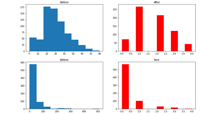

Summary

In this article, we explored different binning techniques used in machine learning. Unsupervised binning methods like equal width and equal frequency binning, as well as k-means binning, were discussed in terms of their definitions, formulas, and advantages. We also implemented these methods using Python's scikit-learn library to demonstrate their practical application. Binning helps to handle outliers and improve model performance by transforming continuous data into discrete intervals, making it a valuable tool in data preprocessing.