
📚What is Quantization in Deep Learning?
Why do we need Quantization?
Let's talk about quantization in deep learning. Have you ever wondered why quantization is important, especially in deep learning? Even though deep learning and large language models (LLMs) are super powerful, they come with many challenges. As these models are large, they can be pretty demanding — they need a lot of computational power and memory, making it tough to use them in places with limited resources. Moreover, they can even use up a lot of energy when making predictions, which makes it become impossible to inference if there is limited computational resource.
Quantization helps deal with these issues by resizing the model to make it more manageable, at the same time be able to reserve almost its performance. This involves revising the number of model parameters and the precision of the data types. By doing this, the models become lighter and faster, which means they can run in more places and use less energy.
The size of a model is calculated by multiplying the number of parameters (size) by the precision of these values (data type).

So the big question is how to reduce the size of the model efficiently. Well, there are a couple of ways to do it. You could reduce the number of parameters or change to lower data type. However, decreasing the number of parameters means making the model smaller and simpler, which is very tricky because it might affect the model's quality substantially. A better option is to tweak how precise the data types are. This is where quantization comes into play — it lets us store model weights in lower-precision formats. This way will help keep the model's effectiveness while making it lighter and faster.
Below are some key reasons why Quantization is crucial in deep learning.
- Efficiency: Quantization reduces the precision of the numerical values in the model, from floating-point to integers. This sounds simple, but it makes the computation a lot easier and faster, which results in speeding things up!
- Memory Savings: By using fewer bits when converting model's weights from floating-point to integers, quantization significantly reduces the size of the models. This is super helpful for deploying models on devices with limited storage and memory, such as smartphones or embedded systems.
- Energy Consumption: As result of smaller model size, we need less computational power to run the models. This is especially helpful if we deploy the model on devices that run on battery.
- Model Deployment: When models are smaller and run faster, it's easier to use them in more places rather than a dedicated big server. This is important for tasks that need quick responses, such as in self-driving cars or real-time translation services.
Types of Quantization
In deep learning, quantization typically involves three main types:
- Post-Training Static Quantization (PTQ): What PTQ is doing is that it shrinks an already trained model (both weights and activations) down without any extra training. It's super straightforward to use, and helps make the model smaller in a short time after finishing training. Just something to keep in mind! Since it does not quantize the model during training, there is chance of a drop in performance compared to the original model.
- Post-Training Dynamic Quantization or Dynamic Quantization: this method trims down the model weights once training is done while handling the activations dynamically on the fly (while inference). This is super handy for models that deal with different types and sizes of inputs. However, keep in mind that since it adjusts the activations live while the model is running, it might slow things down a bit than static quantization. Moreover, another drawback of this method is that not all devices can handle this dynamic approach, so that you have consider when you're planning where to deploy your model with this method.
- Quantization-Aware Training (QAT): The last common method is QAT. This helps keep the model performance by integrating quantization directly into the training process, which can preserve performance better than the other two above by considering quantization effects during model optimization. As the result, QAT asks for a bit more time and energy. It takes longer to train since it's adjusting both learning tasks and quantization at the same time. Plus, it is much more complex to implement. If accuracy is what you require, QAT can make a big difference in keeping your model effective and efficient.
📖Floating number construction
Let's deep-dive into why changing data type reduces model size. When we talk about numbers in computing, it's all about bits — the 0 and 1. This binary encoding system is foundational to computer operations, and different types of numerical representations — like integers and floating-point numbers — have specific ways of organizing these bits.
Integer Representation
For integers, the most common formats are signed and unsigned integers.
Unsigned Integers:
- Bits: All bits represent the magnitude of the number.
- Range: From 0 to 2n-1 (where n is the number of bits).
Signed Integers:
- The first bit is used to tell us if the number is positive (0) or negative (1).
- The rest of the bits show the size of the number or so-called magnitude, where the binary value is inverted and incremented by 1 for negative numbers.
- Range: From -2ⁿ⁻¹ to 2ⁿ⁻¹-1
Floating-Point Representation
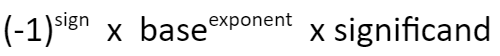
- Sign Bit (1 bit): Indicates the sign of the number; 0 is positive, and 1 is negative.
- Exponent: represents the exponent adjusted by a bias. The actual exponent is calculated by subtracting the bias from the stored exponent. The exponent effectively scales the significant (or mantissa) part of the number by powers of two, allowing floating-point numbers to represent very large or very small values in a compact format.

- Significant/Mantissa: Represents the precision of the number.
Construction of different data types
Float32: uses 32 bits to represent a number:
- 1 bit for the sign
- 8 for the exponent
- The remaining 23 for the significand
- While it provides a high degree of precision, the downside of FP32 is its high computational and memory footprint.
Float16: uses 16 bits to store a number
- 1 is used for the sign
- 5 for the exponent
- 10 for the significand
- Although this makes it more memory-efficient and accelerates computations, the reduced range and precision can introduce numerical instability, potentially impacting model accuracy.
You might be familiar with hearing that float is often called "full precision" (4 bytes), while float16 is "half-precision" (2 bytes).
Common lower precision data types
There are 2 common ways to perform quantization:
- float32 -> float16
- float32 -> int8
Effect of quantization
Imagine we're dealing with a massive model like BLOOM, which has around 176 billion parameters, float32 results in a model size of 176*10**9 x 4 bytes = 704GB. But if we switch to float16, we're down to 352GB, and with int8, just 176 GB. That's a huge cut in the memory space even though 176GB is still a big challenge for many personal computers.
Quantization from float32 to float16
Switching from float32 to float16 is pretty straightforward because they both use similar ways to represent numbers. However, before implementing quantization, it's recommended to consider a few things:
- Software and Hardware Compatibility: First, check if the package you're using can handle float16. Also, does your hardware support it? Modern GPUs and TPUs, like NVIDIA's Turing and Ampere or Google's TPUs, are great for this because they're built to work well with float16, speeding up both learning and inference processes. However, Intel CPUs have been supporting float16 as a storage type, but computation is done after converting to float32.
- Precision needs: Think about how precise your model needs to be, in other words, how sensitive it is to lower precision. For tasks/models where every tiny detail counts, such as in some medical imaging, dropping to a lower precision like float16 can mean losing vital details, which could affect the model's performance.
Quantization from float32 to int8
Quantization from float32 to int8 is trickier because int8 can only handle 256 different values, which is tiny compared to the massive range that float32 handles — about 4 billion numbers ranging from -3.4e38 to 3.4e38. The challenge is to figure out how to squeeze a specific range of float32 values into the much-constrained space of int8.
Stick around, because we're going to dive deep into how we can tackle quantizing down to int8 effectively.
Methods to perform Quantization to int8
Uniform quantization
This method uses a straightforward linear function to map inputs to outputs. Imagine equally spaced points on a line — uniform quantization will keep them all neatly lined up when transforming them. It's quick and easy, but here's the catch: it might not always preserve the distribution of the data very well if that data isn't evenly spread out to begin with.
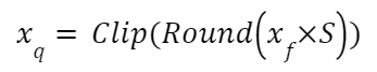
Here's what happens with uniform quantization: it aims to map all the float values between two numbers, let's call them α and β, into a set range [-2ᵇ⁻¹, 2ᵇ⁻¹–1]. If any values fall outside this set range, they're trimmed to the nearest limit — this is what we call clipping.
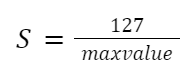
To turn a floating-point number (xf) into an 8-bit representation (xq), we use something called a scale factor (S). This helps match the original data to the new, more compact format of int8, [-128, 127]. And since the zero in the original data will line up with the zero in the new data, we call this symmetric quantization.
How to compute the quantization scale (S)?
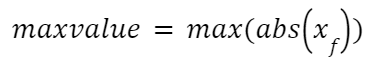
Compute the max value of xf:
Compute the quantization scale (S):
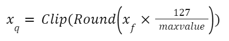
Compute quantized value:
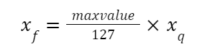
Revert to the original value:
Symmetric quantization treats everything uniformly around zero. This means it evenly handles the ups and downs (positive and negative values) in your data, making sure everything is balanced. It's especially good when your data is zero-centered, or in other words when it spreads out evenly on both sides of zero.
But here's the thing — symmetric quantization might drop the ball when it comes to data that doesn't neatly line up around zero. If your data is more skewed, this method might lead to more quantization errors, since it treats all parts of the range the same.
To solve this issue, we have Non-uniform or Asymmetric quantization, sometimes referred to as Affine Quantization. This technique is a bit more flexible because it adjusts its scale and zero-point differently for different parts of the data, making it a better fit for datasets that are not symmetrically distributed.
Let's try this out with a simple example. We created a weights array with a random normal function from NumPy, hence the array is zero-centered.
# Original weights array
weights = np.random.normal(size = (20000)).astype(np.float32)
weights = torch.from_numpy(weights)
print(weights.mean(), weights.min(), weights.max())
>>> tensor(0.0057) tensor(-3.9224) tensor(4.4791)# Quantize using symmetric method
weights_sym_quant, weights_sym_dequant = symmetric_quantize(weights)
print(weights_sym_quant.double().mean(), weights_sym_quant.double().min(), weights_sym_quant.double().max())
print(weights_sym_dequant.double().mean(), weights_sym_dequant.double().min(), weights_sym_dequant.double().max())
>>> tensor(0.1585, dtype=torch.float64) tensor(-111., dtype=torch.float64) tensor(127., dtype=torch.float64)
>>> tensor(0.0056, dtype=torch.float64) tensor(-3.9148, dtype=torch.float64) tensor(4.4791, dtype=torch.float64)Then we apply the symmetric quantization function, the new quantized array also has an average value of nearly 0, with a min value is -111 and a max value is 127.
Now, we will try to revert the data to the original float range, which is called dequantization. After dequantizing, the average, min, and max values of the dequantized array are approximately equal to the original ones.
Non-uniform quantization
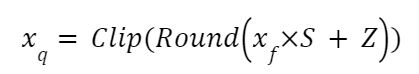
In Asymmetric quantization, an integer is added when computing quantized value. This is called zero-point (Z). Z corresponds to the value 0 in the float32 realm.
Compute quantized value:
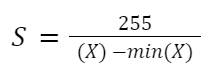
Compute scale (S) value:
Compute zero-point (Z) value:

Asymmetric quantization can handle asymmetric data distributions more effectively by adjusting scale and zero points differently for different parts of the range. However, there are 2 parameters (scale and zero-point), the implementation and optimization process can get complicated, and additional computation power is required during both quantization and dequantization steps.
Asymmetric quantization is great for dealing with uneven data distributions by adjusting the scale and zero points differently across the data range. It's like custom-fitting your data's shoes so they walk more comfortably across the quantization bridge!
But here's the twist: because you're customizing two parameters — scale and zero-point — the setup and fine-tuning can get a bit tricky. Plus, it asks for a bit more computational effort both when quantization and dequantization.
# Quantize using asymmetric method - Normal distribution data
weights_assym_quant, weights_assym_dequant = assymmetric_quantize(weights)
print(weights_assym_quant.double().mean(), weights_assym_quant.double().min(), weights_assym_quant.double().max())
>>> tensor(-8.8287, dtype=torch.float64) tensor(-128., dtype=torch.float64) tensor(127., dtype=torch.float64)
>>> tensor(0.0056, dtype=torch.float64) tensor(-3.9207, dtype=torch.float64) tensor(4.4808, dtype=torch.float64)We saw an example with a normal distribution array, but this is an easy case. Let's try with a trickier one, non-normal distribution.
# Create non-normal distribution data
skewed_weights = np.random.exponential(scale=2, size=20000) - 7 # Shift the data to have both negative and positive values
skewed_weights = torch.from_numpy(skewed_weights)
print(skewed_weights.mean(), skewed_weights.min(), skewed_weights.max())
>>> tensor(-5.0192, dtype=torch.float64) tensor(-6.9999, dtype=torch.float64) tensor(16.4827, dtype=torch.float64)# Quantize using symmetric method
weights_sym_quant, weights_sym_dequant = symmetric_quantize(skewed_weights)
print(weights_sym_quant.double().mean(), weights_sym_quant.double().min(), weights_sym_quant.double().max())
>>> tensor(-38.6737, dtype=torch.float64) tensor(-54., dtype=torch.float64) tensor(127., dtype=torch.float64)As this distribution is not normal, the average value of quantized weights is -38.67, min is -54 and max is 127. The problem here is the whole range of int8 is not fully utilized as the minimum value is only -64. This means the quantization isn't making the most out of the bits available. This might also result in higher quantization errors, as many distinct values might get rounded off to the same quantized value, losing uniqueness and detail in the data.
When we dequantize the weights back to float, the average reaches approximately the value of the original weights.
# Quantize using asymmetric method - Non-normal distribution data
weights_assym_quant, weights_assym_dequant = assymmetric_quantize(skewed_weights)
print(weights_assym_quant.double().mean(), weights_assym_quant.double().min(), weights_assym_quant.double().max())
>>> tensor(-106.5096, dtype=torch.float64) tensor(-128., dtype=torch.float64) tensor(127., dtype=torch.float64)Let's talk about what happens when we turn those quantized values back into their original float range. It's pretty interesting to see that the values from the symmetric method don't spread out quite as evenly as they did in the original data, unlike those from the asymmetric method.
📝Code implementation
Let's work on the quantization example with Pytorch Quantization.
We will use the MobileNetV2 model and MINIST dataset for this demonstration. You can find the details about the dataset here, and how to load the dataset here..
In order to quantize MobileNetV2, we need to implement some modifications in the network.
- The torch.add in InvertedResidual block is replaced with nn.quantized.FloatFunctional()
- self.skip_add = torch.add()
+ self.skip_add = nn.quantized.FloatFunctional()- A fuse_model() method is added to combine Conv+BN and Conv+BN+Relu modules before quantization, enhancing the model's efficiency by reducing memory access and boosting numerical accuracy. This practice is common with quantized models.
class MobileNetV2(nn.Module):
    def __init__(self, num_classes=10, width_mult=1.0, inverted_residual_setting=None, round_nearest=8):
+     self.quant = QuantStub()
+     self.dequant = DeQuantStub()
The general flow to quantize the model using the Pytorch framework is as follows:
# Fuse Conv+BN and Conv+BN+Relu modules prior to quantization (This operation does not change the numerics)
    def fuse_model(self, is_qat=False):
        fuse_modules = torch.ao.quantization.fuse_modules_qat if is_qat else torch.ao.quantization.fuse_modules
        for m in self.modules():
            if type(m) == ConvBNReLU:
                fuse_modules(m, ['0', '1', '2'], inplace=True)
            if type(m) == InvertedResidual:
                for idx in range(len(m.conv)):
                    if type(m.conv[idx]) == nn.Conv2d:
fuse_modules(m.conv, [str(idx), str(idx + 1)], inplace=True)- Configure how an operator should be observed using QConfig. In this code, we use a simple min/max observer to determine quantization parameters.
quantized_model.qconfig = torch.ao.quantization.default_qconfig2. Prepare: insert the Observer/FakeQuantize modules to the model based on specified qconfig
torch.ao.quantization.prepare(quantized_model, inplace=True)3. Calibrate the model to determine quantization parameters for weights and activations. This is done with the training dataset.
evaluate(quantized_model, criterion, data_loader, neval_batches=num_calibration_batches)4. Convert the calibrated model to a quantized model.
torch.ao.quantization.convert(quantized_model, inplace=True)We will load the pretrained model for the MNIST dataset as the original model, quantize this model and compare the results in both size and performance. Performance is evaluated using Top 1 and Top 5 Accuracy.
👑Results👑
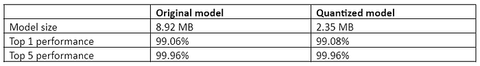
It's pretty amazing how much the model size reduced — from 8.9MB all the way to 2.35MB. That's nearly a 4x reduction! 🌟
When it comes to how well it performs, both the Top 1 and Top 5 accuracy of the quantized model are on-par with the original even though we are using a straightforward min/max observer to pick the quantization parameters. So, we're seeing some promising results without taking up nearly as much space!
Let's check the result of another observer to see how it performs compared to this one. The new observer will determine the quantization parameters automatically.
Instead of using default_qconfig, we will set the configuration to x86 architectures. This architecture quantizes weights on a per-channel basis and then uses a histogram to collect a histogram of activations and optimally picks quantization parameters. The rest of the flow remains the same.
per_channel_quantized_model.qconfig = torch.ao.quantization.get_default_qconfig('x86')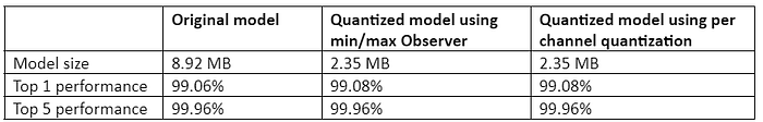
The same result is observed with the new quantization architecture with both Top 1 and Top 5 performance maintains strong output. And the best part? It manages to keep the model size just about the same as with other quantization methods.
Notebook: Link
📕 Final Thoughts
Wrapping up, Post-Training Dynamic Quantization is a handy and efficient trick to optimize machine learning models for deployment. It works by tweaking the weights and activations after all the training is done while able to ensure an acceptable, sometimes on-par performance with the original float model. If you're looking to make your AI projects quicker and leaner, this method could be a real game-changer!
References
https://pytorch.org/docs/stable/quantization.html
MNIST license for commercial use: GNU General Public License v3.0. Link