One Hidden Layer NN

We will build a shallow dense neural network with one hidden layer, and the following structure is used for illustration purpose.

Before trying to understand this post, I strongly suggest you to go through my pervious implementation of logistic regression, as logistic regression can be seem as a 1-layer neural network and the basic concept is actually the same.

Where in the graph above, we have an input vector x = (x_1, x_2), containing 2 features and 4 hidden units a1, a2, a3 and a4, and output one value y_1 in [0, 1].(consider this a binary classification task with a prediction of probability)

In each hidden unit, take a_1 as example, a linear operation followed by an activation function is conducted. So given input x = (x_1, x_2), inside node a_1, we have:

Here w_{11} denotes weight 1 of node 1, w_{12} denotes weight 2 of node 1. Same for node a_2, it would have:

And same for a_3 and a_4 and so on …

Vectorization of One Input

Now let's put the weights into matrix and input into a vector to simplify the expression.

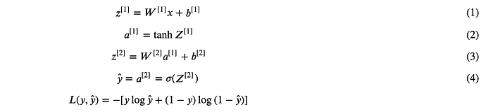
Here we've assumed that the second activation function to be tanh and the output activation function to be sigmoid (note that superscript [i] denotes the ith layer).

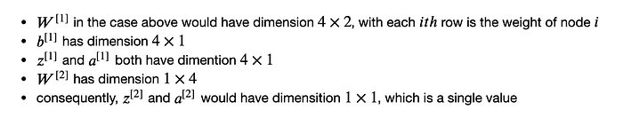
For the dimension of each matrix, we have:

The loss function L for a single value would be the same as logistic regression's (detail introduced here).

Function tanh and sigmoid looks as below.

Notice that the only difference of these functions is the scale of y.

Formula of Batch Training

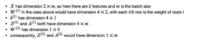
The above shows the formula of a single input vector, however in actual training processes, a batch is trained instead of 1 at a time. The change applied in the formula is trivial, we just need to replace the single vector x with a matrix X with size n x m, where n is number of features and m is the the batch size — samples are stacked column wise, and the following result matrix are applied likewise.

For the dimension of each matrix taken in this example, we have:

Same as logistic regression, for batch training, the average loss for all training samples.

This is all for the forward propagation. To activate our neurons to learn, we need to get derivative of weight parameters and update them use gradient descent.

But now it is enough for us to implement the forward propagation first.

Generate Sample Dataset

Here we generate a simple binary classification task with 5000 data points and 20 features for later model validation.

Weights Initialization

Our neural network has 1 hidden layer and 2 layers in total(hidden layer + output layer), so there are 4 weight matrices to initialize (W^[1], b^[1] and W^[2], b^[2]). Notice that the weights are initialized relatively small so that the gradients would be higher thus learning faster in the beginning phase.

Forward Propagation

Let's implement the forward process following equations (5) ~ (8).

Loss Function

Following equation (9), the loss of each batch can be calculated as following.

Back Propagation

Now it comes to the back propagation which is the key to our weights update. Given the loss function L we defined above, we have gradients as follows:

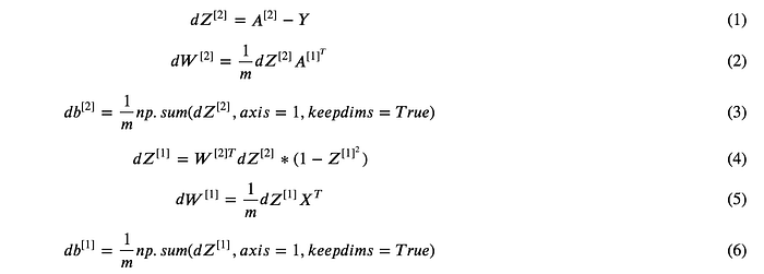
If you are confused that why the derivative of Z^[2] is as above, you can check here. In fact the last layer of our network is the same as logistic regression, so the derivative is inherited from there.

In equation (4), it is element-wise multiplication, and the gradient of tanh{x} is 1 — x². You can try to deduct the equation above by yourself, but I basically took it from internet.

Let's break down the shape of each element, given number of each layer equals (n_x, n_h, n_y) and batch size equals m:

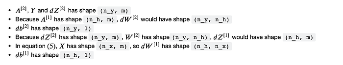
Once we understand the formula, implementation should come with ease.

Batch Training

I have stacked each part into a class, so that it could train like a general package of python. In addition batch training is also implemented. To avoid redundancy, I didn't put it here, for detailed implementation, please check my git repo.

Let's see how our implemented NN performs on our dataset.

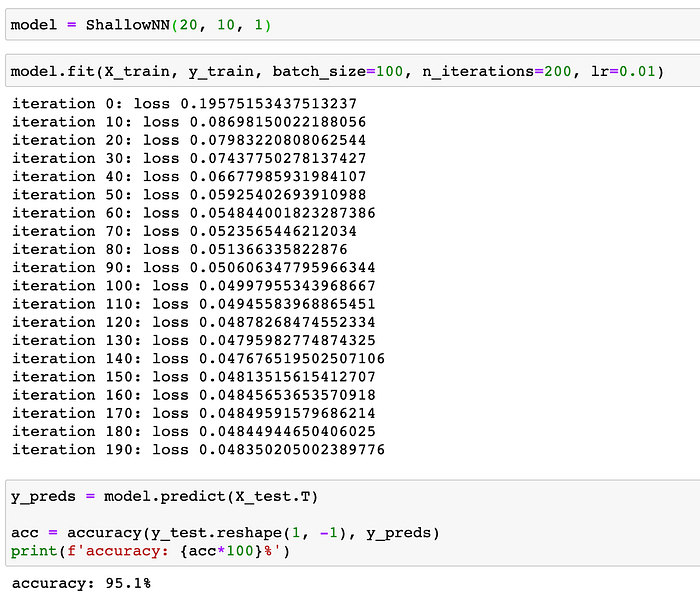
With 10 hidden neurons, our model is able to achieve 95.1% accuracy on test set, which is pretty good.

Now go ahead and try implement yourself, the process would really help you to gain a deeper understanding of general dense neural network.