NLP is a rapidly evolving field that relies heavily on machine learning techniques and deep neural networks. To master this field, understanding the fundamental components of neural networks, such as activation functions, loss functions, and optimizers, is crucial. In this blog post, we'll delve into the world of Python programming and showcase code snippets that illustrate the functioning and applications of these essential components in deep learning. Let's get started!!

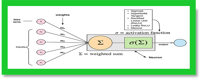
A. Activation Functions: Activation functions are used in artificial neural networks to introduce non-linearity into the model, enabling it to learn and represent complex relationships between inputs and outputs. Here are three commonly used activation functions in Python with simple explanations:

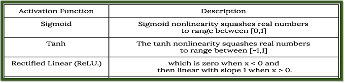
1. ReLU (Rectified Linear Unit): ReLU outputs the input if it's positive and 0 otherwise. It's computationally efficient and helps avoid the vanishing gradient problem.

import numpy as np

def relu(x):
    return np.maximum(0, x)

# Sample input
x = np.array([-1, 0, 1, -2])

# Apply ReLU activation
result = relu(x)

print(result)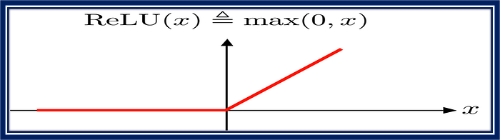

This code snippet defines a function called relu in Python, which calculates the rectified linear unit (ReLU) activation of a given input x. ReLU is a popular activation function in deep learning, that sets all negative values to 0 and leaves the positive values unchanged.

The code then generates an array of input values (x), applies the ReLU function to these values, and stores the results in the result array. Finally, the code prints the resulting array.

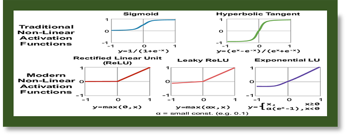
2. Sigmoid: Sigmoid outputs a value between 0 and 1 for any real-valued input. It's useful for problems where the output should be a probability or a value between 0 and 1.

import numpy as np

def sigmoid(x):
    return 1 / (1 + np.exp(-x))

print(sigmoid(0))        # 0.5
print(sigmoid(2))        # 0.88
print(sigmoid(-3))       # 0.05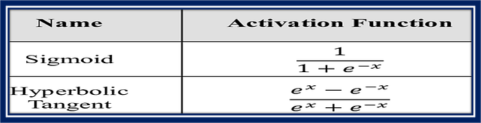

This code snippet defines a function called sigmoid in Python, which calculates the sigmoid function of a given input x. The sigmoid function is an S-shaped curve, and it is commonly used in deep learning as an activation function for neural network layers.

The code then prints the sigmoid function's output for three different input values: 0, 2, and -3. These specific input values are chosen to demonstrate the sigmoid function's behavior, as the output for 0 is approximately 0.5 (half-activated), 2 results in a highly activated output close to 1, and -3 results in a weakly activated output close to 0.

3. tanh (Hyperbolic Tangent): tanh is similar to sigmoid but outputs a value between -1 and 1. It's also used in neural networks but is less popular than ReLU and sigmoid.

import numpy as np

# Define a function for hyperbolic tangent
def tanh(x):
    return np.tanh(x)

# Generate some input values
x = np.array([-2, -1, 0, 1, 2])

# Compute the hyperbolic tangent of the input values
result = tanh(x)

# Print the results
print(result)

This code snippet defines a function called tanh in Python, which calculates the hyperbolic tangent of a given input x. It then generates an array of input values (x), passes those values to the tanh function, and stores the results in the result array. Finally, the code prints the resulting array.

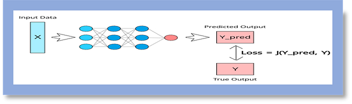
B. Losses: Loss functions are used to evaluate the difference between the predicted output and the true output in a neural network. Here are three commonly used loss functions in Python with simple explanations:

1. MSE (Mean Squared Error): MSE measures the average squared difference between true values (y_true) and predicted values (y_pred). It's a popular choice for regression problems.

import numpy as np

def mse(y_true, y_pred):
    return np.mean((y_true - y_pred) ** 2)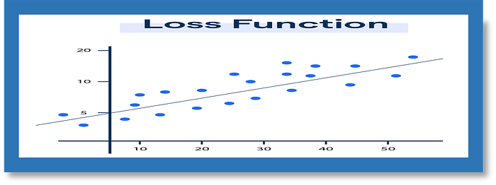

This code snippet defines a function called mse in Python, which calculates the mean squared error (MSE) loss for a given set of true values (y_true) and predicted values (y_pred).

The function calculates the loss by first subtracting the true values from the predicted values, squaring the differences, and then taking the mean of the squared errors.

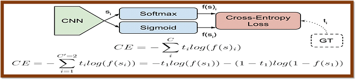
2. Cross-Entropy Loss: Cross-entropy is a commonly used loss function for classification problems. It measures the difference between the predicted probabilities and the true labels.

import numpy as np

def cross_entropy(y_true, y_pred):
    return -np.mean(y_true * np.log(y_pred + 1e-8) + (1 - y_true) * np.log(1 - y_pred + 1e-8))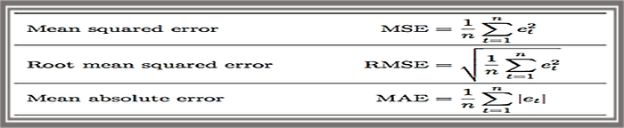

This code snippet defines a function called cross_entropy in Python, which calculates the cross-entropy loss for a given set of true labels (y_true) and predicted probabilities (y_pred).

The function calculates the loss by first multiplying the true labels by the logarithm of the predicted probabilities (with a small added epsilon to avoid numerical instability when taking the logarithm of zero). For the false labels, it multiplies the (1 — true labels) by the logarithm of the predicted complement probabilities (1 — y_pred), also with the added epsilon. Then, it sums the resulting products and takes the negative average.

3. Categorical Cross-Entropy: Categorical cross-entropy is a variant of cross-entropy used for multi-class classification problems. It calculates the cross-entropy for each sample and then averages them.

import numpy as np

def categorical_cross_entropy(y_true, y_pred):
    return -np.mean(np.sum(y_true * np.log(y_pred + 1e-8), axis=1))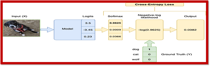

This code snippet defines a function called categorical_cross_entropy in Python, which calculates the categorical cross-entropy loss for a given set of true labels (y_true) and predicted probabilities (y_pred).

The function calculates the loss by first multiplying the true labels by the logarithm of the predicted probabilities (with a small added epsilon to avoid numerical instability when taking the logarithm of zero). Then, it sums the resulting products along the specified axis (in this case, axis=1), and finally, it takes the negative average of this sum.

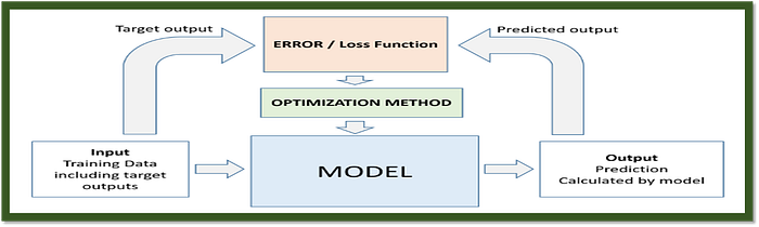
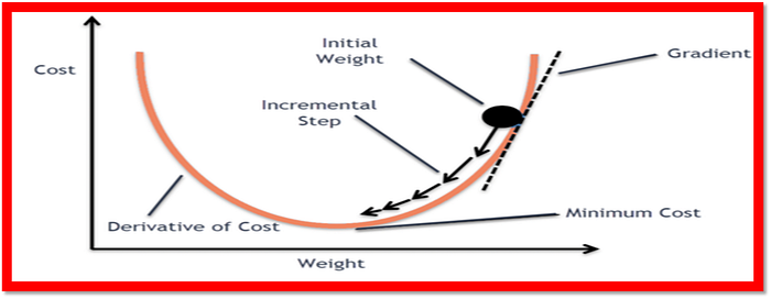
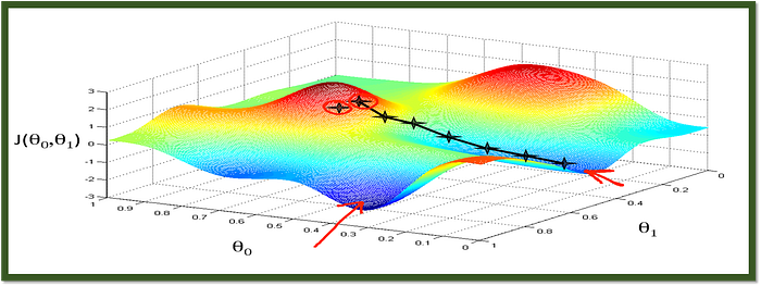
C. Optimizers: Optimizers, also known as learning algorithms, are used to adjust the model's parameters (weights and biases) based on the calculated loss. Here are four commonly used optimizers in the context of artificial neural networks along with their python codes.

1. Gradient Descent: Gradient descent is a simple optimization algorithm that iteratively updates the weights (theta) to minimize the loss. The learning rate (alpha) determines the step size in the weight space.

import numpy as np

def gradient_descent(theta, X, y, alpha):
    theta = theta - alpha * np.dot(X.T, (np.dot(X, theta) - y)) / len(y)
    return theta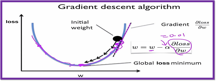

This code snippet defines a function called gradient_descent in Python, which performs gradient descent optimization on a set of parameters (theta). The function takes four arguments: theta, which are the initial model parameters, X, which is the design matrix, y, which is the target vector, and alpha, which is the learning rate.

The function updates the model parameters by subtracting the product of the learning rate, the gradient of the cost function, and the transpose of the design matrix, divided by the number of data points in the target vector, from the original parameters. The gradient of the cost function is calculated by taking the dot product of the design matrix and the original parameters and subtracting the target vector.

2. Momentum: Momentum adds a velocity term to the weight updates, which helps the optimization escape local minima and converge faster. The learning rate (alpha) and the decay rate (beta) can be adjusted to control the optimization.

import numpy as np

class MomentumOptimizer:
    def __init__(self, alpha=0.01, beta=0.9):
        self.alpha = alpha
        self.beta = beta
        self.velocity = 0

    def update(self, theta):
        self.velocity = self.beta * self.velocity + self.alpha * np.gradient(cost)
        theta -= self.velocity
        return theta

This code snippet defines a custom Momentum Optimizer class in Python, which is used to optimize the parameters of a deep learning model. The Momentum Optimizer class has two instance variables, alpha and beta, which are the learning rate and a momentum factor, respectively. It also has an instance variable, velocity, used to store the current momentum.

The update method is used to adjust the model parameters (theta) based on the current momentum, the learning rate, and the gradient of the cost function. It updates the momentum by multiplying the previous momentum with the momentum factor and adding the new gradient scaled by the learning rate. Then, it updates the model parameters by subtracting the new momentum from the original weights.

3. Nesterov Accelerated Gradient (NAG): NAG is a variant of momentum that estimates the gradient using the predicted weights instead of the current weights. This can help the optimization converge faster.

import numpy as np

class NAGOptimizer:
    def __init__(self, alpha=0.01, beta=0.9):
        self.alpha = alpha
        self.beta = beta
        self.velocity = 0

    def update(self, theta):
        # Predict the new weights based on the velocity and the learning rate
        theta_pred = theta - self.velocity * self.alpha
        self.velocity = self.beta * self.velocity + self.alpha * np.gradient(cost, theta_pred)
        theta -= self.velocity
        return theta

This code snippet defines a custom NAG Optimizer class in Python, which is used to optimize the parameters of a deep learning model. The NAG Optimizer class has two instance variables, alpha and beta, which are the learning rate and a momentum factor, respectively. It also has an instance variable, velocity, used to store the current momentum.

The update method is used to adjust the model parameters (theta) based on the current momentum, the learning rate, and the gradient of the cost function. It first predicts the new weights by subtracting the current momentum scaled by the learning rate from the original weights. Then, it updates the momentum using the previous momentum and the new gradient scaled by the learning rate and the momentum factor. Finally, it updates the model parameters using the new momentum.

4. Adam Optimizer: Adam (Adaptive Moment Estimation) is a widely used optimization algorithm that adapts the learning rate for each weight by maintaining separate estimates of the first and second moments of the gradient. This adaptive nature can lead to faster convergence and better performance compared to other optimization methods.

import numpy as np

class AdamOptimizer:
    def __init__(self, alpha=0.001):
        self.alpha = alpha
        self.m = None
        self.v = None
        self.t = 0

    def update(self, gradient):
        self.t += 1
        if self.m is None:
            self.m = gradient
            self.v = gradient * gradient
        else:
            self.m = self.m * 0.999 + gradient * (1 - 0.999)
            self.v = self.v * 0.999 + gradient * gradient * (1 - 0.999)

        m_hat = self.m / (np.sqrt(self.v) + 1e-8)
        self.alpha *= (1 - 0.999) ** self.t
        theta -= self.alpha * m_hat
        return theta

This code snippet defines a custom Adam Optimizer class in Python, which is used to optimize the parameters of a deep learning model. The Adam Optimizer class has a single instance variable, alpha, which is the learning rate. It also has three instance variables, m, v, and t, which are used to store the first and second moments of the gradients, and the iteration number, respectively.

The update method is used to adjust the model parameters (theta) based on the current gradient and the stored moment estimates. The method updates the moment estimates and the iteration count, calculates the update direction using the estimated moments and the learning rate, and updates the model parameters. Finally, it returns the updated model parameters.

Cheers!! Happy reading!! Keep learning!!

Please upvote if you liked this!! Thanks!!

You can connect with me on LinkedIn, YouTube, Kaggle, and GitHub for more related content. Thanks!!