Scalping is one of the most popular intraday trading styles, designed to capture small but frequent price movements throughout the day. Instead of holding positions for hours or days, scalpers aim to profit from quick entries and exits, often within minutes. To succeed with this approach, traders need a reliable tool that adapts to changing market conditions and helps them set realistic targets.

This is where the Average True Range (ATR) indicator comes into play. Originally developed by J. Welles Wilder, ATR is a volatility-based indicator that measures the degree of price movement in an asset. By combining ATR with a scalping strategy, traders can determine optimal stop-loss and take-profit levels, manage risk effectively, and improve their consistency in volatile markets.

In this article, we'll explore how to trade using an ATR based scalping strategy, and how it can help intraday traders achieve more disciplined and profitable trades.

What is ATR (Average True Range)?

The True Range takes into account:

1. The difference between today's high and low.
2. The difference between today's high and yesterday's close.
3. The difference between today's low and yesterday's close.

The ATR value is then calculated as the moving average (commonly 14 periods) of these true ranges.

Common Interpretation:

• A high ATR means the market is volatile, with large price swings.
• A low ATR indicates quiet markets with smaller movements.

For scalpers, this information is crucial. ATR doesn't predict direction, but it provides an objective way to size stop losses and profit targets, ensuring trades align with actual market conditions instead of guesswork.

Why Use ATR for Scalping?

Since traders are targeting small price moves, even a minor mistake in stop-loss or target placement can wipe out several successful trades. This is where the ATR adds value.

Dynamic Risk Management

• ATR helps you avoid setting arbitrary stop losses.
• In a volatile market, stops and targets naturally widen. In calmer conditions, they tighten.
• This ensures you don't get stopped out too early or set unrealistic profit targets.

Adaptability Across Assets

• Whether trading forex, stocks, indices, or commodities, ATR automatically adjusts to the volatility of that instrument.
• Scalpers can use the same principle across markets without rewriting their strategy.

Noise Filtering

• ATR-based levels reduce the impact of small intraday price fluctuations.
• This helps traders avoid overreacting to market noise and focus on meaningful moves.

Consistency in Execution

• By using ATR multiples (e.g., 1× ATR for stop loss, 1.5–2× ATR for targets), traders build repeatable and disciplined trade setups.

Tips to Improve Consistency with ATR Scalping

Even though the ATR-based scalping method is simple, consistency comes from applying the right filters and discipline. Here are some tips:

Combine ATR with a Trend Filter

• Use a moving average to trade with the trend, not against it.
• Avoid scalping in sideways markets where ATR values may be misleading.

Add a Momentum Confirmation

• Check RSI (above 50 for longs, below 50 for shorts) or MACD crossover for entry confirmation.
• This reduces false signals and improves win rate.

Avoid Low-Liquidity Hours

• Scalping works best during high-volume sessions (London & New York overlap, or Indian market open for Nifty/Bank Nifty).
• ATR readings in low liquidity may give false volatility.

Respect Risk Management

• Never risk more than 1–2% per trade.
• Stick to predefined stop-loss and target levels — don't move them impulsively.

Backtest & Forward Test

• Backtest the ATR strategy on your chosen market (Forex, Gold, Indices).
• Try it on a demo account first to build confidence before going live.

These practices ensure you not only take high-probability trades but also maintain the discipline required for consistent intraday profits.

Here is a python code demonstrating use of trend filters along with ATR scalping strategy for XAU/USD trades. In this code 200 SMA, 20 EMA filters and RSI have been used along with ATR

"""
ATR-based scalping strategy with trend filters and backtesting.
Applies ATR stops/targets + 200 SMA trend filter + 20 EMA + RSI confirmation + ATR volatility regime.
"""

import pandas as pd
import numpy as np
import yfinance as yf
import matplotlib.pyplot as plt

# ------------------------------
# Calculate ATR & RSI
# ------------------------------
def calculate_atr(data, window=14):
    """Calculate ATR and True Range."""
    data['tr1'] = data['High'] - data['Low']
    data['tr2'] = abs(data['High'] - data['Close'].shift())
    data['tr3'] = abs(data['Low'] - data['Close'].shift())
    data['TrueRange'] = data[['tr1', 'tr2', 'tr3']].max(axis=1)
    data['ATR'] = data['TrueRange'].rolling(window=window).mean()
    return data

def compute_rsi(series, window=14):
    """Calculate RSI without TA-Lib."""
    delta = series.diff()
    gain = delta.clip(lower=0)
    loss = -delta.clip(upper=0)

    avg_gain = gain.rolling(window=window, min_periods=window).mean()
    avg_loss = loss.rolling(window=window, min_periods=window).mean()

    rs = avg_gain / avg_loss
    rsi = 100 - (100 / (1 + rs))
    return rsi

# ------------------------------
# Strategy
# ------------------------------
def atr_scalping_with_filters(
    data, atr_window=14, sl_multiple=1.0, tp_multiple=2.0, 
    trend_filter_window=200, short_filter_window=20
):
    """ATR scalping with SMA/EMA/RSI filters and volatility regime."""

    # Indicators
    data = calculate_atr(data, window=atr_window)
    data['SMA_long'] = data['Close'].rolling(window=trend_filter_window).mean()
    data['EMA_short'] = data['Close'].ewm(span=short_filter_window).mean()
    data['RSI'] = compute_rsi(data['Close'], window=14)

    data.dropna(inplace=True)
    data.reset_index(inplace=True)

    data['Signal'] = 0
    data['Returns'] = 0.0

    position, entry_price, stop_loss, take_profit = 0, 0, 0, 0

    # Volatility regime thresholds (20th–80th percentile of ATR)
    atr_threshold_low = data['ATR'].quantile(0.2)
    atr_threshold_high = data['ATR'].quantile(0.8)

    for i in range(len(data)):
        row = data.iloc[i]

        # Scalars
        price, o, h, l = float(row['Close']), float(row['Open']), float(row['High']), float(row['Low'])
        atr, tr = float(row['ATR']), float(row['TrueRange'])
        sma_long, ema_short, rsi = float(row['SMA_long']), float(row['EMA_short']), float(row['RSI'])

        # Volatility regime filter
        if atr < atr_threshold_low or atr > atr_threshold_high:
            continue

        if position == 0:
            # Long entry
            if (price > sma_long) and (ema_short > sma_long) and (rsi > 55) and (tr < atr):
                position = 1
                entry_price = price
                stop_loss = price - sl_multiple * atr
                take_profit = price + tp_multiple * atr
                data.at[i, 'Signal'] = 1

            # Short entry
            elif (price < sma_long) and (ema_short < sma_long) and (rsi < 45) and (tr < atr):
                position = -1
                entry_price = price
                stop_loss = price + sl_multiple * atr
                take_profit = price - tp_multiple * atr
                data.at[i, 'Signal'] = -1

        elif position == 1:
            if l <= stop_loss or h >= take_profit:
                exit_price = stop_loss if l <= stop_loss else take_profit
                data.at[i, 'Returns'] = (exit_price - entry_price) / entry_price
                position = 0
                data.at[i, 'Signal'] = 2   # long exit

        elif position == -1:
            if h >= stop_loss or l <= take_profit:
                exit_price = stop_loss if h >= stop_loss else take_profit
                data.at[i, 'Returns'] = (entry_price - exit_price) / entry_price
                position = 0
                data.at[i, 'Signal'] = -2  # short exit

    return data

# ------------------------------
# Performance Summary
# ------------------------------
def performance_summary(data):
    trades = data[data['Returns'] != 0]
    num_trades = len(trades)
    win_trades = trades[trades['Returns'] > 0]
    win_rate = (len(win_trades) / num_trades * 100) if num_trades > 0 else 0
    avg_return = trades['Returns'].mean() * 100 if num_trades > 0 else 0
    total_return = (1 + trades['Returns']).prod() - 1
    total_return_pct = total_return * 100

    # Max Drawdown
    cum_returns = (1 + trades['Returns']).cumprod()
    peak = cum_returns.cummax()
    drawdown = (cum_returns - peak) / peak
    max_dd = drawdown.min() * 100 if not drawdown.empty else 0

    print("\n📊 Performance Summary")
    print(f"Total Trades     : {num_trades}")
    print(f"Win Rate         : {win_rate:.2f}%")
    print(f"Average Return   : {avg_return:.2f}% per trade")
    print(f"Total Return     : {total_return_pct:.2f}%")
    print(f"Max Drawdown     : {max_dd:.2f}%")

# ------------------------------
# Plotting
# ------------------------------
def plot_results(data, strategy_name):
    data['Cumulative Returns'] = (1 + data['Returns']).cumprod() - 1
    total_return = data['Cumulative Returns'].iloc[-1] * 100

    # Detect x-axis
    x = data['Datetime'] if 'Datetime' in data.columns else (data['Date'] if 'Date' in data.columns else data.index)

    plt.style.use('seaborn-v0_8-darkgrid')
    plt.figure(figsize=(12, 6))
    plt.plot(x, data['Cumulative Returns'], color='blue', label='Strategy Returns')
    plt.axhline(y=0, color='gray', linestyle='--')
    plt.title(f'{strategy_name} Backtest (Total Return: {total_return:.2f}%)')
    plt.xlabel('Date'); plt.ylabel('Cumulative Return')
    plt.legend(); plt.xticks(rotation=45)
    plt.tight_layout(); plt.show()

# ------------------------------
# Main Run
# ------------------------------
if __name__ == '__main__':
    ticker = 'GC=F'  # Gold Futures proxy for XAU/USD
    start = (pd.to_datetime('today') - pd.DateOffset(years=1)).strftime('%Y-%m-%d')
    end = pd.to_datetime('today').strftime('%Y-%m-%d')

    print(f"Fetching 1 year of data for {ticker}...")
    df = yf.download(ticker, start=start, end=end, interval='1h')

    if df.empty:
        raise ValueError("No data returned from yfinance.")

    print("Running improved ATR strategy with filters...")
    backtest_data = atr_scalping_with_filters(df.copy())

    print("Backtest complete. Generating stats and plot...")
    performance_summary(backtest_data)
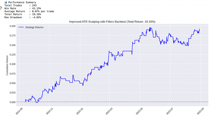
    plot_results(backtest_data, "Improved ATR Scalping with Filters")

Here is the outcome of the backtest

Advantages & Limitations of ATR-Based Scalping

Advantages

Adaptive Risk Management

• ATR automatically adjusts stops and targets to current volatility, keeping trades realistic.

Simplicity

• Easy to implement on any trading platform with minimal indicators.

Cross-Market Usability

• Works well in Forex, commodities, indices, and even liquid stocks.

Consistency

• Using ATR multiples (e.g., 1× stop, 1.5×–2× target) creates a disciplined, repeatable system.

Noise Reduction

• ATR helps filter out market chop and sets levels beyond random fluctuations.

Limitations

Does Not Predict Direction

• ATR only measures volatility, not trend — you still need a filter like EMA/RSI.

Frequent Trades Required

• Scalping needs many trades per session, which can be stressful and spread-sensitive.

Risk of Overtrading

• Small moves may tempt traders to over-leverage, leading to quick losses if discipline slips.

Performance Varies by Market

• ATR scalping works best in highly liquid instruments; in illiquid assets, results may be unreliable.

In short, ATR scalping is a powerful but minimalist approach — best used with trend/momentum confirmation and strict money management.