Introduction

Bootstrap is a method of random sampling with replacement. Among its other applications such as hypothesis testing, it is a simple yet powerful approach for checking the stability of regression coefficients. In our previous article, we explored the permutation test, which is a related concept but executed without replacement.

Linear regression relies on several assumptions, and the coefficients of the formulas are presumably normally distributed under the CLT. It shows that on average if we repeated the experiment thousands and thousands of times, the line would be in confidence intervals. The bootstrap approach does not rely on those assumptions*, but simply performs thousands of estimations. *(Please note, that the bootstrap approach does not violate or bypass the normality assumptions, but rather than relying on the CLT, it builds its own, the Bootstrap distribution, which is asymptotically normal)

In this article, we will explore the Bootstrapping method and estimate regression coefficients of simulated data using R.

Dataset Simulation

We will simulate a dataset of one exploratory variable from the Gaussian distribution, and one response variable constructed by adding random noise to the exploratory variable. The population data would have 1000 observations.

set.seed(2021)
n <- 1000
x <- rnorm(n)
y <- x + rnorm(n)
population.data <- as.data.frame(cbind(x, y))

We will take a sample of 20 observations from these data.

sample.data <- population.data[sample(nrow(population.data), 20, replace = TRUE),]

Simple Regression Models

Let's explore the simple regression models both for population and for sample data:

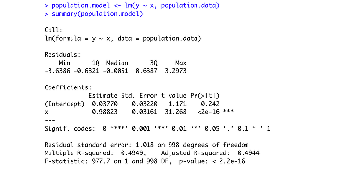
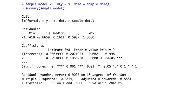
We can see, that the intercept is biased for the sample data; however, the slope coefficient is very close to the population one, even though we have only 20 observations in our sample dataset. The standard errors are much higher for the sample model.

If we plot the models, we can see how close the lines are:

Bootstrap Approach

The Bootstrap approach asks a question: what if we resample the data with replacement and estimate the coefficients, how extreme would it be?

Here is a simple loop of 1000 trials, which resamples with replacement these 20 observations from our sample dataset, runs the regression model and saves the coefficients we get there. In the end, we would have 1000 pairs of coefficients.

We would take the average of these coefficients, and compare them with the other models we previously obtained:

We can see, in this particular example, the intercept is closer to the population model, and the slope is at around the same precision level as the sample model. But what we are more interested, is the precision of confidence intervals.

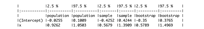
We can see, that the precision is almost identical to the sample model's, and even slightly tighter for the intercept.

The Graphical Representation

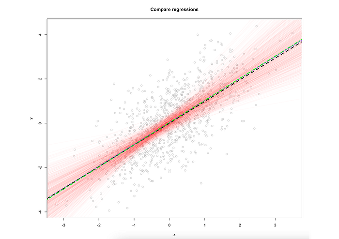
First, the bootstrap representation:

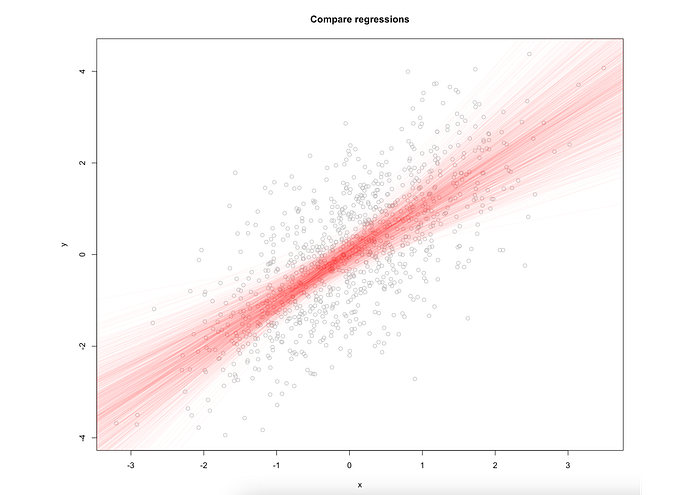
These are 1000 possible regression lines we have estimated. Now let's add to the plot population, sample, and average bootstrap lines:

We can see that they essentially capture the data in the same way. Now let's add the confidence intervals from the sample data:

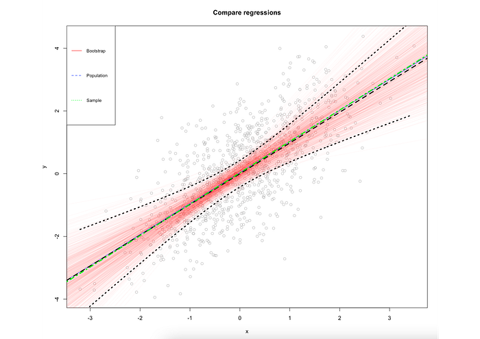
This completes our research: we may conclude, that the bootstrapping approach returns essentially the same results but in a statistically different fashion. We do not rely on assumptions but simulate the data using a brute force method. This could be especially useful when we have doubts about the distribution the data arrived from, or want to check the stability of the coefficients, particularly for small datasets.

You can find the full code here on GitHub.

Conclusion

In this article, we have explored the bootstrap approach for estimating regression coefficients. We used a simple regression model for simplicity and clear representation of this powerful technique. We concluded that this approach is essentially equal to the OLS models, however without relying on the assumptions. It is a powerful method for estimating the uncertainty of the coefficients and could be used along with traditional methods to check the stability of the models.

Thank you for reading!

Connect on LinkedIn