Shiv Gupta
Carlos Fabbri-Garcia
Dany Stefan
Louis D'Hulst
GitHub Repository: https://github.com/shiv-io/connect4-reinforcement-learning
Connect 4: Background
Connect Four is a two-player connection board game, in which the players choose a color and then take turns dropping colored tokens into a seven-column, six-row vertically suspended grid. The pieces fall straight down, occupying the lowest available space within the column. The objective of the game is to be the first to form a horizontal, vertical, or diagonal line of four of one's own tokens.
Reinforcement learning approaches
In this article, we discuss two approaches to create a reinforcement learning agent to play and win the game.
Deep Q Learning
Deep Q Learning is one of the most common algorithms used in reinforcement learning. In it, neural networks are used to facilitate the lookup of the expected rewards given an action in a specific state. To understand why neural network come in handy for this task, lets first consider the more simple application of the Q-learning algorithm
Q-Learning
The Q-learning approach can be used when we already know the expected reward of each action at every step. We can think that we have a "cheat sheet" in the form of the table, where we can look up each possible action under a given state of the board, and then learn what is the reward to be obtained if that action were to be executed. The idea of "total reward", which is a combination of the next immediate reward and the sum of all the following ones, is also called the Q-value.
The Q-learning approach may sound reasonable for a game with not many variants, e.g. tic-tac-toe, where keeping a table to condense all the expected rewards for any possible state-action combination would take not more that one thousand rows perhaps. However, when games start to get a bit more complex, there are millions of state-action combinations to keep track of, and the approach of keeping a single table to store all this information becomes unfeasible. In the case of Connect4, according to the online Encyclopedia of Integer Sequences, there are 4,531,985,219,092 (4 quadrillion) situations that would need to be stored in a Q-table. Most present-day computers would not be able to store a table of this size in their hard drives.
Also, even with long training cycles, we won't always guarantee to show the agent the exhaustive list of possible scenarios for a game, so we also need the agent to develop an "intuition" of how to play a game even when facing a new scenario that wasn't studied during training. For these reasons, we consider a variation of the Q-learning approach, which is the Deep Q-learning.
Deep Q-learning
In deep Q-learning, we use a neural network to approximate the Q-value functions. The state of the environment is passed as the input to the network as neurons and the Q-value of all possible actions is generated as the output. Please consider the diagram below for a comparison of Q-learning and Deep Q-learning
*Source: AnalyticsVidhya
To train a deep Q-learning neural network, we feed all the observation-action pairs seen during an episode (a game) and calculate a loss based on the sum of rewards for that episode. For example, if winning a game of connect-4 gives a reward of 20, and a game was won in 7 steps, then the network will have 7 data points to train with, and the expected output for the "best" move should be 20, while for the rest it should be 0 (at least for that given training sample).
If we repeat these calculations with thousands or millions of episodes, eventually, the network will become good at predicting which actions yield the highest rewards under a given state of the game. Most importantly, it will be able to predict the reward of an action even when that specific state-action wasn't directly studied during the training phase. Also, the reward of each action will be a continuous scale, so we can rank the actions from best to worst.
Of course, we will need to combine this algorithm with an explore-exploit selector so we also give the agent the chance to try out new plays every now and then, and expand the lookup space. For that, we will set an epsilon-greedy policy that selects a random action with probability 1-epsilon and selects the action recommended by the network's output with a probability of epsilon. The idea is to reduce this epsilon parameter over time so the agent starts the learning with plenty of exploration and slowly shifts to mostly exploitation as the predictions become more trustable.
#Define epsilon decision function
def epsilonDecision(epsilon):
  action_decision = random.choices(['model','random'], weights = [1 - epsilon, epsilon])[0]
  return action_decision
epsilonDecision(epsilon = 0) # would always give 'model'
Connect 4 Kaggle Environment
By now we have established that we will build a neural network that learns from many state-action-reward sets. So, we need to interact with an environment that will provide us with that information after each play the agent makes. In other words, we need to have an opponent that will allow the network understand if a move (or game) was played well (resulting winning) or bad (resulting in losing). For that we will take advantage of a Connect-4 environment made available by Kaggle for a past Reinforcement Learning competition.
from kaggle_environments import evaluate, make, utils
import gym
env = make("connectx", debug=True)
env.render()
#Creates a new random trainer
trainer = env.train([None, 'negamax'])
#Resets the board, shows initial state of all 0
trainer.reset()['board']
#Make a new action: play position 4
new_obs, winner, state, info = trainer.step(4)
Every time we interact with this environment, we can pass an action as input to the game. After that, the opponent will respond with another action, and we will receive a description of the current state of the board, as well as information whether the game has ended and who is the winner. As long as we store this information after every play, we will keep on gathering new data for the deep q-learning network to continue improving.
Experimenting with the neural network
We built a notebook that interacts with the Connect 4 environment API, takes the output of each play and uses it to train a neural network for the deep Q-learning algorithm.
During the development of the solution, we tested different architectures of the neural network as well as different activation layers to apply to the predictions of the network before ranking the actions in order of rewards. One of the experiments consisted of trying 4 different configurations, during 1000 games each:
- Experiment 1: Last layer's activation as linear, don't apply softmax before selecting best action
- Experiment 2: Last layer's activation as ReLU, don't apply softmax before selecting best action
- Experiment 3: Last layer's activation as linear, apply softmax before selecting best action
- Experiment 4: Last layer's activation as ReLU, apply softmax before selecting best action
We compared the 4 options by trying them during 1000 games against Kaggle's opponent with random choices, and we analyzed the evolution of the winning rate during this period. We also verified that the 4 configurations took similar times to run and train.
As shown in the plot, the 4 configurations seem to be comparable in terms of learning efficiency. All of them reach win rates of around 75%-80% after 1000 games played against a randomly-controlled opponent. For the purpose of this study, we decide to keep the experiment 3 as the best one, since it seems to be the one with the steadier improvement over time.
The Code
Creating the Deep Learning Model
The first step in creating the Deep Learning model is to set the input and output dimensions. There are 7 different columns on the Connect 4 grid, so we set num_actions to 7. We set the input shape to [6,7] and reshape the Kaggle environment output in order to have an easier time visualizing the board state and debugging.
#Number of possible actions
num_actions = 7
#Number of different states
num_states = [6,7]
The next step is creating the models itself. For this we are using the TensorFlow Functional API. Note that while the structure and specifics of the model will have a large impact on its performance, we did not have time to optimize settings and hyperparameters. Each layers uses a ReLu activation function except for the last, which uses the linear function. This is based on the results of the experiment above.
# Create the DQN
input = tf.keras.layers.Input(shape = (num_slots))
flatten = tf.keras.layers.Flatten()(input)
hidden_1 = tf.keras.layers.Dense(50, activation = 'relu')(flatten)
hidden_2 = tf.keras.layers.Dense(50, activation = 'relu')(hidden_1)
hidden_3 = tf.keras.layers.Dense(50, activation = 'relu')(hidden_2)
hidden_4 = tf.keras.layers.Dense(50, activation = 'relu')(hidden_3)
output = tf.keras.layers.Dense(num_actions, activation = "linear")(hidden_4)
model = tf.keras.models.Model(inputs = [input], outputs = [output])
Creating Needed Functions
We now have to create several functions needed to train the DQN. The first of these, getAction, uses the epsilon decision policy to get an action and subsequent predictions. The model predictions are passed through a softmax activation function before being returned.
def getAction(model, observation, epsilon):
  #Get the action based on greedy epsilon policy
  action_decision = epsilonDecision(epsilon)
  #Reshape the observation to fit in model
  observation = np.array([observation])
  #Get predictions
  preds = model.predict(observation)
  #Get the softmax activation of the logits
  weights = tf.nn.softmax(preds).numpy()[0]
  if action_decision == 'model':
    action = np.argmax(weights)
  if action_decision == 'random':
    action = random.randint(0,6)
  return int(action), weights
The model needs to be able to access the history of the past game in order to learn which set of actions are beneficial and which are harmful. This is why we create the Experience class to store past observations, actions and rewards. The class has two functions: clear(), which is simply used to clear the lists used as memory, and store_experience, which is used to add new data to storage. Note that this is not an optimal way of storing data for the model to learn from, and would certainly run into efficiency issues if the model was trained for a significant length of time.
class Experience:
  def __init__(self):
    self.clear()
  def clear(self):
    self.observations = []
    self.actions = []
    self.rewards = []
  def store_experience(self, new_obs, new_act, new_reward):
    self.observations.append(new_obs)
    self.actions.append(new_act)
    self.rewards.append(new_reward)
The next function is used to cover up a potential flaw with the Kaggle Connect4 environment. It is possible, and even fairly likely, for a column to be filled to the top during a game. Placing another piece in that column would be invalid, however the environment still allows you to attempt to do so. We therefore have to check if an action is valid before letting it take place.
This is done by checking if the first row of our reshaped list format has a slot open in the desired column. If it doesn't, another action is chosen randomly. There are most likely better ways to do this, however the model should learn to avoid invalid actions over time since they result in worse games.
# Check if action is valid
# #Requires reshape(6,7) format
def checkValid(obs, action):
  valid_actions = set([0,1,2,3,4,5,6])
  if obs[0,action] != 0:
    valid_actions = valid_actions - set([action])
    action = random.choice(list(valid_actions))
  return action
Rewards also have to be defined and given. This is done through the getReward() function, which uses the information about the state of the game and the winner returned by the Kaggle environment. Four different possible outcomes are defined in this function. The first checks if the game is done, and the second and third assign a reward based on the winner. The final outcome checks if the game is finished with no winner, which occurs surprisingly often. We set the reward of a tie to be the same as a loss, since the goal is to maximize the win rate. Note that we were not able to optimize the reward values.
#Function to get reward
def getReward(winner, state):
  #Game not done wet
  if not state:
    reward = 0
  if state:
    #If player 1 wins
    if winner == 1:
      reward = 50
    #If player 2 wins
    if winner == -1:
      reward = -50
    if winner == 0:
      reward = -50
  return reward
The final function uses TensorFlow's GradientTape function to back propagate through the model and compute loss based on rewards. Weights are computed by the model using every observation from a game, and softmax cross entropy is then performed between the set of actions and weights. Finally, we reduce the product of the cross entropy values and the rewards to a single value: model loss.
def train_step(model, optimizer, observations, actions, rewards):
    with tf.GradientTape() as tape:
      #Propagate through the agent network
        logits = model(observations)
        softmax_cross_entropy = tf.nn.sparse_softmax_cross_entropy_with_logits(logits=logits, labels=actions)
        loss = tf.reduce_mean(softmax_cross_entropy * rewards)
        grads = tape.gradient(loss, model.trainable_variables)
        optimizer.apply_gradients(zip(grads, model.trainable_variables))
Training the model
We are now finally ready to train the Deep Q Learning Network. To do so we must first create the environment, define an optimizer (in our case Adam), initialize an Experience object, and set our initial epsilon value and its decay rate. We are then ready to start looping through the episodes. In our case, each episode is one game. Note that we use TQDM to track the progress of the training. TQDM may not work with certain notebook environments, and is not required.
Each episode begins by setting up a trainer to act as player 2. We trained the model using a random trainer, which means that every action taken by player 2 is random. This was done for the sake of speed, and would not create an agent capable of beating a human player. In the ideal situation, we would have begun by training against a random agent, then pitted our agent against the Kaggle negamax agent, and finally introduced a second DQN agent for self-play. The Kaggle environment is not ideal for self-play, however, and training in this fashion would have taken too long.
After creating player 2 we get the first observation from the board and clear the experience cache. We can then begin looping through actions in order to play the games. The first step is to get an action and then check if the it is valid. Once we have a valid action, we play it using trainer.step() and retrieve new data about the board, the state of the game and the reward. Most rewards will be 0, since most actions do not end the game. The final while loop checks if the game is finished. If it is, we can train our agent using the train_step() function and play the next game.
#Train P1 (model) against random agent P2
#Create the environment
env = make("connectx", debug=True)
#Optimizer
optimizer = tf.keras.optimizers.Adam()
#Set up the experience storage
exp = Experience()
epsilon = 1
epsilon_rate = 0.995
wins = 0
win_track = []
for episode in tqdm.tqdm(range(10000)):
  #Set up random trainer
  trainer = env.train([None, 'random'])
  #First observation
  obs = np.array(trainer.reset()['board']).reshape(6,7)
  #Clear cache
  exp.clear()
  #Decrease epsilon over time if we want
  epsilon = epsilon * epsilon_rate
  #Set initial state
  state = False
  while not state:
    #Get action
    action, w = getAction(model, obs, epsilon)
    #Check if action is valid
    while True:
      temp_action = action
      action = checkValid(obs, temp_action)
      if temp_action == action:
        break
    #Play the action and retrieve info
    new_obs, winner, state, info = trainer.step(action)
    obs = np.array(new_obs['board']).reshape(6,7)
    #Get reward
    reward = getReward(winner, state)

    #Store experience
    exp.store_experience(obs, action, reward)
    #Break if game is over
    if state:
      #This would be where training step goes I think
      if winner == 1:
        wins += 1
      win_track.append(wins)
      train_step(model2, optimizer = optimizer,
                 observations = np.array(exp.observations),
                 actions = np.array(exp.actions),
                 rewards = exp.rewards)
      break
Monte Carlo Tree Search
This approach speeds up the learning process significantly compared to the Deep Q Learning approach. Monte Carlo Tree Search (MCTS) excels in situations where the action space is vast. In the case of Connect 4, the action space is 7. As such, to solve Connect 4 with reinforcement learning, a large number of permutations and combinations of the board must be considered.
Monte Carlo Tree Search builds a search tree with n nodes with each node annotated with the win count and the visit count. Initially the tree starts with a single root node and performs iterations as long as resources are not exhausted.
There are 4 steps to a MCTS algorithm.
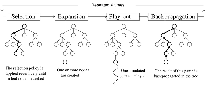
- Initial Setup — Start with a single root (parent) node and assign a large random UCB value to each non visited (child) nodes.
- Selection — In this phase, the agent starts at the root node, selects the most urgent node, applies the selected action, and continues until the final state is reached. To select the most urgent node, the upper limit of the node's trust limit is used. The node with the largest UCB is used as the next node. The UCB process helps overcome the dilemma of exploration and exploitation. Also known as the multi-armed bandit problem, agents want to maximize their prizes during gambling (lifelong learning).

- Expansion — When UCB can no longer be applied to find the next node, the game tree is expanded further to include unexplored child by appending all possible nodes from the leaf node.
- Simulation — Once expanded the algorithm selects the child node either randomly or with a policy until it reaches the final state of the game.
- Backpropagation — When the agent reach the final state of the game with a winner, all the traversed node are updated. The visit and win score for each nodes are updated.
The above steps are repeated for some iterations. Finally the child of the root node with the highest number of visits is selected as the next action as more the number of visits higher is the ucb.
The algorithm steps:
- Each iteration starts at the root
- Follows tree policy to reach a leaf node
- Node 'N' is added
- Perform a random rollout
- Value backpropagated up the tree
How the algorithm learns:
- Agents require more episodes to learn than Q-learning agents, but learning is much faster.
- For simplicity, both trees share the same information, but each player has its own tree. We have found that this method is more rigorous and more flexible to learn against other types of agents (such as Q-Learn agents and random agents).
- It takes about 800MB to store a tree of 1 million episodes and grows as the agent continues to learn. Therefore, it goes far beyond CNN to remain constant throughout the learning process.