In this article (and the next few), we will discuss in detail how to train multi-layered perceptrons efficiently.

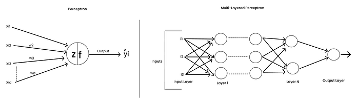
But before that, let's first understand how to train a single-neuron model — the Perceptron ; before scaling up to a multi-layered perceptron.

What Does Training a Neural Network Mean?

What does "training" mean in general for any machine learning algorithm?

To answer this, let's go back to what we discussed earlier — "the goal of learning is to capture the pattern from the given data."

For any ML algorithm, we have certain parameters that we need to fine-tune to best capture these patterns in the dataset. If we encounter similar unseen data during inference, the model should be able to classify or predict correctly.

This idea applies to neural networks as well.

Unlike traditional algorithms that capture simple linear or non-linear relationships, neural networks can model complex patterns through:

• Multiple interconnected layers.
• Non-linear activation functions.
• Optimization techniques (to tune parameters effectively).

Why Do We Optimize Weights in Neural Networks?

In neural networks, the inputs come from the dataset, and we cannot change them.

So the only way to make the network learn better is by adjusting the weights and biases.

Since activation functions are predefined and remain fixed once chosen, the main elements to optimize are:

• The weights Wi's.
• The biases bi's.
• The learning rate η, which controls the update step size.

Thus, training a network means optimizing weights and biases so that the network performs best on both training and unseen data.

Finally, we are on point now, we need to find optimal weights and biases in order to have a best learning network. This mean training network will be to optimize weights and biases.

From Perceptron to Linear and Logistic Regression

Let's start simple,

The Perceptron and Logistic Regression are both single-neuron models for classification. Linear Regression, on the other hand, is a single-neuron model for regression.

Linear Regression as a Single Neuron Model

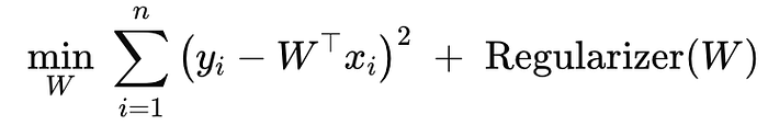
In Linear Regression, the goal is to find the optimal weights W's and bias b that minimize the squared loss.

In Linear Regression :

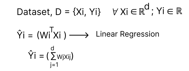
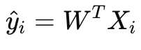
Here the task is to find the optimal "W", intercept.

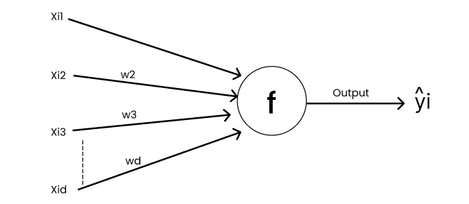
So, now the input to "F" in Fig is

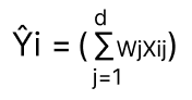
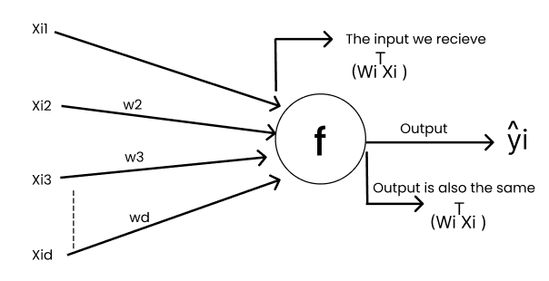
In this Linear Regression "f" is an Identity Function.

[Identity function is to express an input in a function in terms of input itself; F(z) = z]

In the case of Logistic Regression it is a Sigmoid/Logistic Function.

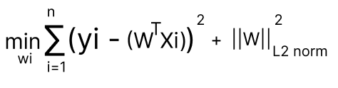
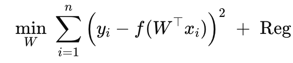
In Linear Regression, our optimization task we write it as find wi's that minimize loss function which is squared loss.

Single Neuron — Perceptron:

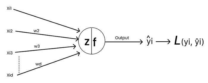
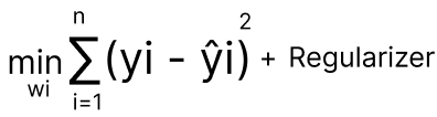
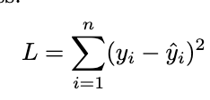
Defining Loss Function

yi is the ground truth & ŷi is the predicted output.

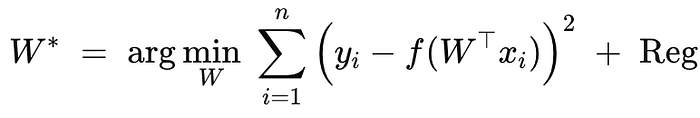
Optimization Problem we have,

Find wi,

W* → Optimal w.

Identity Function → Linear Regression.

Sigmoid Function → Logistic Regression.

Step Function → Perceptron.

for vector w →

Solving the Optimization Problem

SGD: Stochastic Gradient Descent

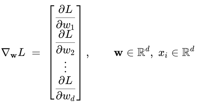
1. Initialization of weights, wi's → Randomly.
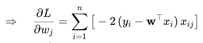
2. Gradient vector (derivative w.r.t. w):

3. Update rule (learning rate η):

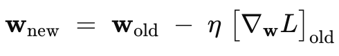
For-loop: iterations t →1 to K till convergence.

Gradient Descent vs Stochastic Gradient Descent

GD: ∇wL uses all {xi,yi}; i=1 →n

SGD: ∇w​L≈ gradient from one point (x(i),y(i)) or a small batch (mini-batch, which is popular.

Let Fi ≡ f (w⊤xi); ŷ​i​=Fi​

Loss = L

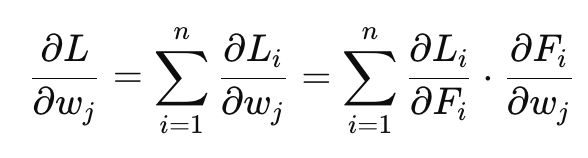
Gradient via Chain Rule:

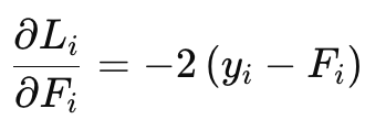
For Squared Loss:

Training an Multi-Layered Perceptron: Introduction to Back Propagation

Training a Multi-Layered Perceptron using Stochastic Gradient Descent with Chain Rule.

Loss Function → Squared Loss.

Assume our task is a regression problem, so that we can handle the numerical values. We have Xi's which are inputs Yi's which are ground truth in our dataset.

Now, How does a Neural Network looks like?

It looks like the following way with weights, activation functions and biases.

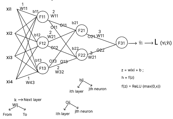
Let's say we have a fully connected neural network with multiple connections across its layers. Each input has a set of weights that are initially randomly initialized, these are the parameters we need to optimize during training.

Each input is multiplied by its corresponding weight and then passed through an activation function (for example, ReLU, which acts as a positive-only gate). The output from this activation becomes the input to the next layer, where it's again multiplied by new weights and passed through another activation function. This process continues layer by layer until we reach the output layer, which produces the predicted output.

This entire flow is called Forward Propagation, it computes the network's initial output based on the inputs and the current (random) weights. Once we get this output, we compare it with the ground truth and use that difference (loss) to optimize the weights in the next step.

So, this is it? Do we have our expected output?

No, it is of course a predicted output, it is no close to the original ground truth that we already have within our dataset. Now, since we have the predicted output and the ground truth we will compute the loss through a Loss function.

Note: Every connection will have a weight.

Loss Function is Squared Loss.

What is Loss? What is Loss Function?

Loss in terms of Machine Learning/ Deep Learning is how far the trained model is from the ground truth. This can be computed with equation called "Loss Function." Loss Function is a function that will help us to compute how good a model is working.

Note: In this case, we are working on a regression problem and the loss -function is a squared loss.

But how are we going to optimize the weights based on the loss function value?

We did forward propagation and at the end we had output and computed loss using loss-function. So, now we will come back to optimize each and every weight based on that loss.

This backward process of updating weights is called "Backward Propagation."

Optimizing the Networks

In the beginning part of this article we have seen that training a neural network is to find the optimized weights within each connections.

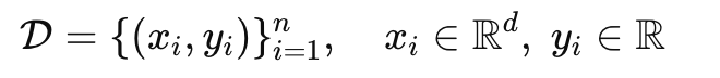
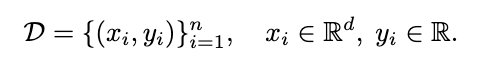
Let's Say we have the dataset

Step 1 : Initialize weights randomly

Each input vector xi passes through multiple layers of the neural network to produce an output ŷi

Step2 : For each Xi in D-Train, compute forward propagation

The structure of an MLP consists of fully connected layers. Each neuron in layer l computes:

where f is an activation function (e.g., ReLU, Sigmoid, Tanh)

Activation Example (ReLU) :

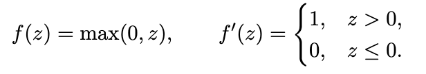
ReLU acts as a positive-only gate, allowing gradients to flow through non-negative regions.

Forward Pass Intuition:

During the forward pass,

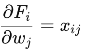
→Inputs xi are multiplied with corresponding weights wij .

→ Each layer applies the activation function to produce Oj(l)

→The final output layer produces ŷi, the prediction for input xi.

This process is called Forward Propagation. It computes the predicted output given initial (random) weights.

Compute Loss using a Loss-Function

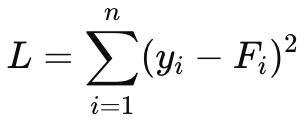
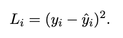
To measure prediction error, we use the Squared Loss.

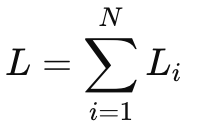
Here, L represents how far the model's predictions are from the true ground truth values. Each individual loss is

Note: The measure of loss quantifies how well the model performs.

Backward Propagation:

After forward propagation, the model has computed ŷi. But since the loss is still high initially, we must adjust the weights.

Backward Propagation (Backprop) is the process of computing how much each weight contributed to the overall loss and updating it accordingly. This is done using the Chain Rule of Calculus. We propagate the loss backward from the output layer to the input layer.

Step4: Compute all the derivatives using Chain rule and use it efficiently by tricks like memoization.

The goal is to minimize:

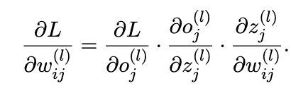
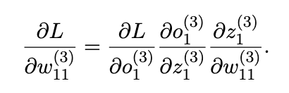
To find how each weight affects L, we compute:

Output Layer Example:

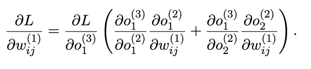
Input Layer Example:

If a weight multiple paths, this is how you compute derivatives

Step 5: Update weights from the end of the network to the beginning → Backward Propagation.

Each weight wij(l) is updated based on its gradient:

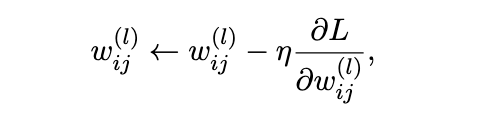
where,

η is the learning rate.

The updates proceed in reverse order:

Output Layer → Hidden Layers → Input Layer.

[update nth layer, then n-1 layer, then n-2 layer and so….on 1st layer]

Summary : We will send the inputs to the network as a forward pass (or) propagation computes the loss through loss function. Once we have the loss we can find the derivatives. So, that we can update these weights.

First we will update the third layer weights, then the second layer and then first layer.

[update nth layer, then n-1 layer, then n-2 layer and so….on 1st layer]

Intuitively whats happening here is that in forward propagation we will compute the error rate of the model. In the backward propagation we will use that error rate and based on that rate we will optimize the weights.

So, for the next input batch the weights will be a bit better than the previous one and the error-rate will be declined.

Step 3: Repeat the step-2 until convergence.

Memoization in Back-propagation:

During back-propagation, we compute gradients of the loss function with respect to every weight in the network. For each weight, these gradients depend on the chain of derivatives from the subsequent layers.

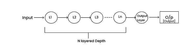
For example,

• When optimizing layer L1​ weights, we require gradient information from layers L2, L3,…,Ln​ (all layers ahead of it).
• Similarly, when optimizing layer L2​, we need derivatives from L3,L4,…,Ln and so on.

Why Memoization?

Since these derivatives are reused multiple times while updating weights across layers, recomputing them for each connection would be redundant and computationally expensive.

Instead, we can compute the derivatives once, store them in memory, and reuse them wherever required during that iteration.

This process of storing intermediate results to avoid redundant re-computation is known as Memoization.

Mathematical Representation

In back-propagation, we use the chain rule to propagate gradients backward

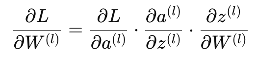
Now, the partial term ∂L/∂a(l) depends on the gradient from the next layer l+1:

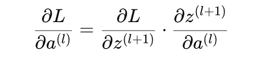
Since this term will be reused for all neurons connected to a(l), we compute it once and store it in memory (memoization) rather than recalculating it multiple times.

Efficiency Gain

Using memoization:

• Reduces redundant gradient computations.
• Saves significant time and computational power.
• Increases the efficiency of each training iteration (especially in deep networks).

Thus, the back-propagation process can be viewed as:

Back-propagation → Chain Rule + Memoization.

Epochs and Multi-Epoch Training

An epoch is defined as sending the entire training dataset through the network once — performing both forward and backward passes.

• If the dataset is passed once → 1 Epoch
• If it's passed five times → 5 Epochs

Formally, for a dataset:

D = { (Xi,Yi) ∣ i = 1, 2, …, N }

One complete pass of all samples D through the model constitutes one epoch.

Back-propagation intuitively

1. Step 1: Initialize the weights randomly.
2. Step 2: Perform the forward pass, compute activations layer by layer.
3. Step 3: Perform the backward pass, compute gradients using the chain rule and store intermediate derivatives using memoization.
4. Step 4: Update/Adjust/optimize weights using the computed gradients.
5. Step 5: Repeat for multiple epochs until convergence.

Note: Back-Propagation works if and only if the activation functions are differentiable.

If activation functions are not differentiable, we cannot leverage back-propagation.

Since, all the outputs within the network 011, 012, 013, 021, 022, 031 are from the activation functions, and we cannot differentiate the activation functions we cannot use them in the back-propagation. If Fij 's are not differentiable we can't have chain rule for updating and because if there are only constants everything will be "0" and no weight updation no matter how many epochs.

If the activation functions are easily differentiable, it will speed up the training of the Neural Networks using Back-Propagation.

In the network we can see there is an input layer multiple hidden layers one output layer and a prediction.

Instead of Sending one input through the network, it is better to send a batch of points through the network to speed up the process.

From the perspective of Gradient Descent

What does Gradient Descent do?

It takes all the points and find the derivatives and use it in the convergence.

What Does Stochastic Gradient Descent Do?

Stochastic Gradient Descent (SGD) takes one data point at a time, computes its derivatives, and uses them to move the parameters toward convergence.

xi ⇒ SGD update.

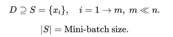
What Does Mini-Batch Stochastic Gradient Descent Do?

Mini-batch SGD takes a subset of data points (a batch) at a time, computes their derivatives, and approximates convergence using the batch's averaged gradient.

Why Mini-Batch Training?

Keeping the entire dataset in RAM and computing derivatives using all data points simultaneously is extremely time-consuming. Hence, most implementations prefer mini-batch or single-sample (SGD) updates over full-batch training.

Mini-batch based back-propagation is the most popular and efficient approach in deep learning.

So, people will prefer a single-point based back-prop (or) mini-batch based back-prop over total datapoints to compute back-prop.

Example:

Suppose there are 10,000 samples in the dataset. Mini-batch size=100.

Then:

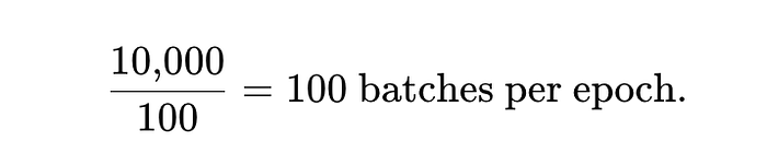
For each mini-batch of 100 samples:

• Perform forward propagation
• Compute loss using a loss function
• Find derivatives (gradients)
• Update weights through backpropagation

Instead of running 10,000 individual updates, we now run just 100, making the process far more efficient.

Overview:

Mini-batch back-propagation strikes a balance between:

• The accuracy of full-batch gradient descent, and
• The speed of stochastic updates.

It is the standard training method used in almost all modern neural networks. So, mini-batch based back-prop is famous for all sorts of neural networks.

Conclusion

To wrap it up, training a neural network, whether it's a simple perceptron or a multi-layered model like deep neural networks, it is all about optimizing the weights and biases so that the predicted values will be as close as possible to the actual ground truth that we already have in our dataset.

In forward propagation, we do the dot product of the weights and inputs from the data through the network to get the predicted output. Then, in backward propagation, we adjust each weight using the chain rule figuring out how much every weight contributed to the overall error. To make this process faster and more efficient, we use memoization, so that the computed derivatives are stored once and reused instead of recalculated again and again, for the sake of efficiency.

As we repeat this process over multiple epochs, the network gradually learns, the loss reduces, and the predictions will improve. In practice, mini-batch back-propagation strikes a perfect balance between speed and accuracy, which is why it's used almost everywhere in modern deep learning.

At its core, back-propagation = chain rule + memoization, a combination of math and efficiency that powers how every neural network learns and evolves through data.