This is the 2nd article of my "Point Cloud Processing" tutorial. "Point Cloud Processing" tutorial is beginner-friendly in which we will simply introduce the point cloud processing pipeline from data preparation to data segmentation and classification.

• Article 1 : Introduction to Point Cloud Processing
• Article 2 : Estimate Point Clouds From Depth Images in Python
• Article 3 : Understand Point Clouds: Implement Ground Detection Using Python
• Article 4 : Point Cloud Filtering in Python
• Article 5 : Point Cloud Segmentation in Python

In the previous tutorial, we introduced point clouds and showed how to create and visualize them. In this tutorial, we will learn how to compute point clouds from a depth image without using the Open3D library. We will also show how the code can be optimized for better performance.

Table of contents:
· 1. Depth Image
· 2. Point cloud
 ∘ 2.2 Depth camera calibration
 ∘ 2.3 Point cloud computing
· 3. Colored point cloud
· 4. Code optimization
 ∘ 4.1 Point cloud
 ∘ 4.2 Colored point cloud
· 5. Conclusion

1. Depth Image

A depth image (also called a depth map) is an image where each pixel provides its distance value relative to the sensor's coordinate system. Depth images can be captured by structured light or time-of-flight sensors. To compute depth data, structured light sensors, such as Microsoft Kinect V1, compare the distortion between projected and received light. As for time-of-flight sensors like Microsoft Kinect V2, they project light rays and then compute the time elapsed between the projection and the reception of these later.

In addition to the depth image, some sensors provide their corresponding RGB image to form an RGB-D image. The latter makes it possible to compute a colored point cloud. This tutorial will use the Microsoft Kinect V1 RGB-D image as an example.

Let's start by importing the libraries:

Now, we can import the depth image and print its resolution and its type:

Image resolution: (480, 640)
Data type: int32
Min value: 0
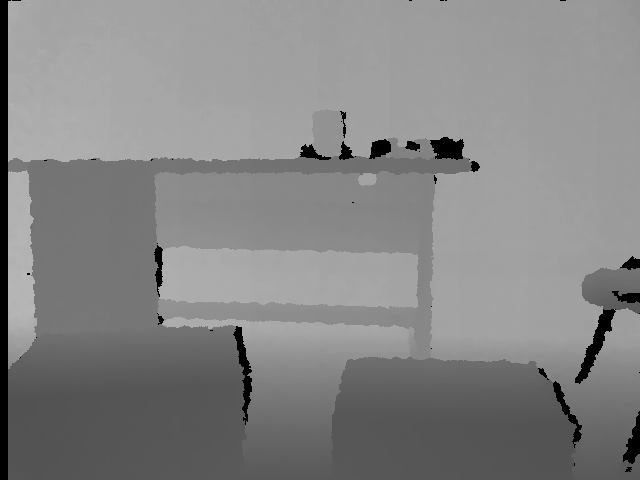
Max value: 2980

The depth image is a matrix of size 640×480 where each pixel is a 32 (or 16) bit integer that represents the distance in millimeters and for this reason the depth image looks black when opened (see figure below). The min value 0 represents the noise (there is no distance) while the max value 2980 represents the distance of the farthest pixels.

For a better visualization, we compute its grayscale image:

Computing the grayscale image means scaling the depth values to [0, 255]. Now the image is clearer now:

Note that, Matplotlib does the same thing when visualizing the depth image:

2. Point cloud

Now that we have imported and displayed the depth image, how can we estimate the point cloud from it? The first step is to calibrate the depth camera to estimate the camera matrix and then use it to compute the point cloud. The obtained point cloud is also called 2.5D point cloud since it is estimated from a 2D projection (depth image) instead of 3D sensors such as laser sensors.

2.2 Depth camera calibration

Calibrating a camera means estimating lens and sensor parameters by finding the distortion coefficients and the camera matrix also called the intrinsic parameters. In general, there are three methods for calibrating a camera : using the standard parameters provided by the factory, using the results obtained in calibration research or calibrating the Kinect manually. Calibrating the camera manually consists of applying one of the calibration algorithm such as the chess-board algorithm[1]. This algorithm is implemented in Robot Operating System (ROS) and OpenCV. The calibration matrix M is a 3×3 matrix:

Where fx, fy and cx, cy are the focal length and the optical centers respectively. For this tutorial, we will use the obtained results of NYU Depth V2 dataset:

If you want to calibrate the camera yourself you can refer to this OpenCV tutorial.

2.3 Point cloud computing

Computing point cloud here means transforming the depth pixel from the depth image 2D coordinate system to the depth camera 3D coordinate system (x, y and z). The 3D coordinates are computed using the following formulas [2], where depth(i, j) is the depth value at the row i and column j:

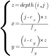
The formula is applied for each pixel:

Let's display it using Open3D library:

3. Colored point cloud

What if we want to compute the colored point cloud from an RGB-D image? The color information can enhance the performance of many tasks like point cloud registration. In this case, if the input sensor provides the RGB image too, it is preferable to use it. A colored point cloud can be defined as follows:

Where x, y and z are the 3D coordinates and r, g and b represent the color in the RGB system.

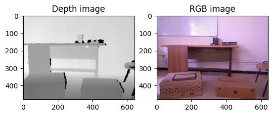
We start by importing the corresponding RGB image of the previous depth image:

To find the color of a given point p(x, y,z) that is defined in the depth sensor 3D coordinate system:

1. We transform it to the RGB camera coordinate system [2]:

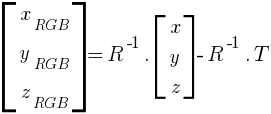
Where R and T are the extrinsic parameters between the two cameras: the rotation matrix and the translation vector respectively.

Similarly, we use the parameters from NYU Depth V2 dataset:

The point in the RGB camera coordinate system is computed as follows:

2. Using the intrinsic parameters of the RGB camera, we map it to color image coordinate system [2]:

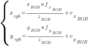
These are the indices to get the color pixel.

Note that in the previous formulas, the focal length and the optical centers are the RGB camera parameters. Similarly, we use the parameters from NYU Depth V2 dataset:

The indices of the corresponding pixel is computed as follows:

Let's put all together and display the point cloud:

4. Code optimization

In this section, we explain how to optimize your code to be more efficient and suitable for real-time applications.

4.1 Point cloud

Computing point clouds using nested loops is time consuming. For a depth image with 480×640 as resolution, on a machine having 8GB RAM and an i7–4500 CPU, computing the point cloud took about 2.154 seconds.

To reduce the computation time, nested loops can be replaced by vectorisation operations and the computation time can be reduced to about 0.024 seconds:

We can also reduce the computation time to about 0.015 seconds by computing the constant once at the beginning:

4.2 Colored point cloud

As for the colored point cloud, on the same machine, executing the previous example took about 36.263 seconds. By applying vectorisation, the running time is reduced down to 0.722 seconds.

5. Conclusion

In this tutorial, we learned how to compute point clouds from RGB-D data. In the next tutorial, we will closely analyze the point clouds by taking a simple ground detection as an example.

Thanks, I hope you enjoyed reading this. You can find the examples here in my GitHub repository.

References

[1] Zhang, S., & Huang, P. S. (2006). Novel method for structured light system calibration. Optical Engineering, 45(8), 083601.

[2] Zhou, X. (2012). A Study of Microsoft Kinect Calibration. Dept. of Computer Science, George Mason University, Fairfax.

Image credits

All images and figures in this article whose source is not mentioned in the caption are by the author.