

In the previous posts, we have discussed Regression and Support Vector Machines (SVM) as two important methods in Machine Learning. SVM has some similarity to a Regression Analysis, however, there is a method that is a direct descendent of a Logistic Regression. It is called 'Artificial Neural Network (ANN)'. We shall build an ANN from scratch in this article, and you would be able to understand the concept with an interactive tool.
Introduction
The history of Artificial Neural Networks goes back to the early decades of the 20th century. It was an inspiration from the biological neurons which form network(s) in a human brain. An Artificial Neural Network (ANN) is a collection of neurons which are connected in layers, and which produces an output when the neurons in the input layer are excited. A very simple depiction of an artificial neuron is shown in the following figure.
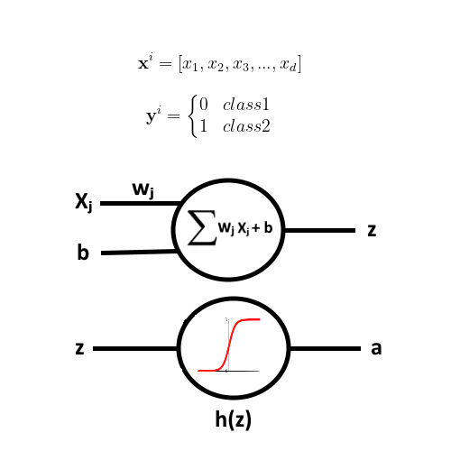
An Artificial Neuron has a number of inputs Xⱼ and weights Wⱼ. Based on what neuron receives at the input, it outputs a single value Z which is the dot product of the vector Wⱼ with Xⱼ. There is also a bias term b which is added as a linear combination to the dot-product. If you recall Regression from our earlier lesson, then you would understand why this is the case. It is the linear combination representing a linear Regression function with weights Wⱼ and inputs Xⱼ. The output of a Neuron is mapped onto a range by applying an activation function (e.g., Sigmoid). Such an activation function adds non-linearity to the output and keeps it within a range (e.g., 0–1).
Network Construction
The Artificial Neurons, which were explained in the previous section, are connected, and arranged in a set of multiple layers. A very simple ANN consists of three layers: An input layer (⁰L), a hidden layer (¹L), and an output Layer (²L). The input layer consists of the values Xⱼ and the output layer provides the result of the network which is the probability of the output class for the given inputs. The number of neurons in the output layer depends on the number of classes in the dataset. In the following figure such a simple 3-Layer ANN is displayed.
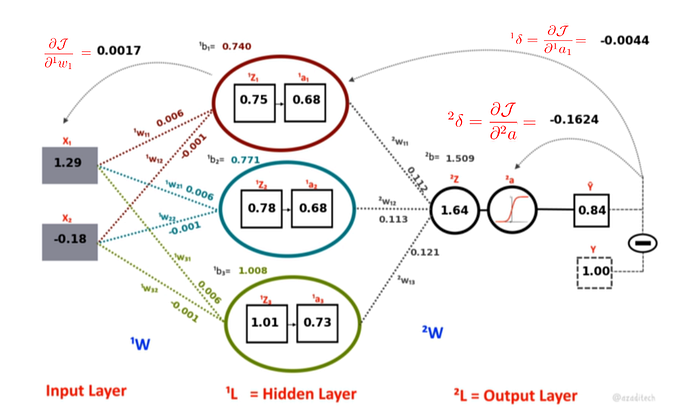
The learning takes place in between the layers. More specifically, the weights ˡW at each layer 'l' are learned such that the output resembles the true class label when these weights are plugged-in the ANN. The weights ˡW are arranged in the form of matrices, one for each layer transition. The dimension of a weight matrix ˡW depends on the number of neurons in the layer 'l' and the number of neurons in the previous layer. The number of inputs is considered as number of Neurons for layer Ɔ'.
The neurons in all the layers have two components: the output value computed from the dot-product of the weights with the inputs and the outputs of the activation functions. In the example shown in figure 3, we have only one output which means, it only produces probability of a single class. The activation function (i.e. Sigmoid) in the last layer makes sure that the values remain between 0 and 1. It is important to note here the resemblance of this simple network with a Logistic Regression. In-fact, a simple 3-Layer network with a single hidden layer like in the figure 3 is nothing but a linear Logistic Regression which would only work best for linearly separable data. One must add multiple hidden layers in order to add non-linearity to the system.
Objective Function Formulation
ANN poses an optimization problem, like any other machine learning method, it seeks to optimize an objective function over a set of parameters for obtaining the desired output. More specifically, we are trying to find the best values for weights w such that when we plug them into an ANN it should output the true class label yᶦ for the input Xᶦ. We achieve this by minimizing the error (ŷ — y) where ŷ is the predicted class probability by the ANN while the y is the true class label. In practice, we compute such error by taking log of the ŷ and arrange it in a linear combination for accommodating the both the Ƈ' labels and the Ɔ' labels. The objective function is shown in the figure 4 below.
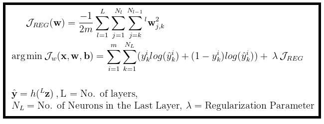
If you paid attention, you would notice that there is another term JREG added to the objective function as well. This is for a Regularization term to ensure that model avoids overfitting. It is the square sum of all the weights in all the layers. The lambda parameter is the tradeoff between the Regularization and the accuracy over the training-set. The lower values may make a model form a tight decision boundary on the training-set and thus might fail to accommodate new variant examples in the test-set, while a large value might cause model to not be fit enough for the data.
Feed-Forward Process
A Neural Network consists of two types of processes: the feed-forward process, and the backpropagation process. The feed-forward process is responsible for computing the outputs for the individual neurons in the network based on the respective inputs and the weight of the neurons. More specifically, the values of ˡz are computed for each Neuron in the network by taking linear combination of respective weights ˡw, input activations from the previous layer ˡ⁻¹a and biases ˡb. The values of ˡz are then transformed into activations ˡa by applying the activation functions. The complete list of operations performed in a feed-forward process are shown in figure 5.

Backpropagation Process
Perhaps the key to learning lies in the backpropagation step of an ANN. It is the step which follows the feed-forward step and it is responsible for distributing the error to each of the weights in the network. A backpropagation step begins by computing the error (ŷ — y) at the last layer of the network. This error is then used to compute the change in the weights at each layer. This is accomplished by applying the chain rule of the partial derivatives. Recall from your calculus that f(g(x)) = f'(g(x)).g'(x). Now backtrack from the output to the input in such a way that you end up computing the change in objective function w.r.t the weights (∂J/∂w). This can be computed by backtracking the partial derivatives w.r.t to the outputs in the current layer and multiplying them with the outputs at the previous layer. The partial derivative w.r.t outputs can be further decomposed using chain-rule until we reach the layer 0. These partial derivatives are depicted as deltas in figure 6. The computed deltas are then multiplied recursively with the activations at each previous layer starting from the last layer. You may also notice a derivative of the sigmoid function multiplied as well while calculating the delta, this is because we computed activations by applying the sigmoid function on the outputs of the neurons (i.e., a = h(z)).
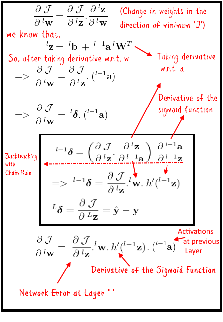
Notice also how we computed the change in outputs z w.r.t the weights w (∂J/∂w). We used the definition of the z and took a derivative of z w.r.t the w. We did the same thing for computing the partial derivative of z at the current layer w.r.t the a activations at the previous layer (∂ˡz/∂ˡ⁻¹a). The only difference is that we took the derivative of z w.r.t the ˡ⁻¹a this time.
We compute these partial derivatives of J w.r.t. w at each layer and obtain a gradient matrix ˡw' for each weight matrix ˡw. These gradient matrices represent the change in the value of each weight in the direction of the optimum value of J. An optimizer (e.g., Gradient Descent) then uses these gradients to update the weights (e.g., wₙ = w — α w'), where α is the learning rate.
Implementation in Python
We construct a simple Neural Network from scratch for this Lesson using only numpy in python. The network consists of three layers: the input layer, one hidden layer, and an output layer. The input takes two-dimensional data (kept it simple for understanding the concept). There are three Neurons in the hidden layer. The output layer has one Neuron which outputs the probability of the input point for being from the class. Full ANN is shown in figure 3 along with weights, biases, outputs, and activations of each Neuron.
Linear Classification
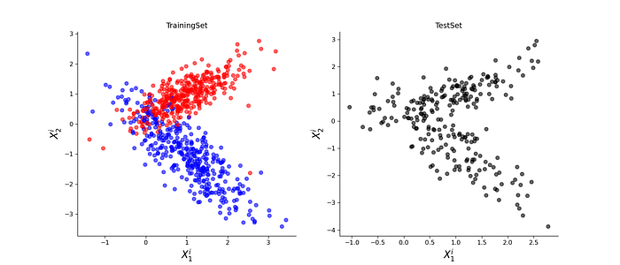
The constructed Network can be used to classify a set of data points belonging to two classes (0/1). We construct a random set of data points and then split it into a training and a test split. This can be seen from figure 7.
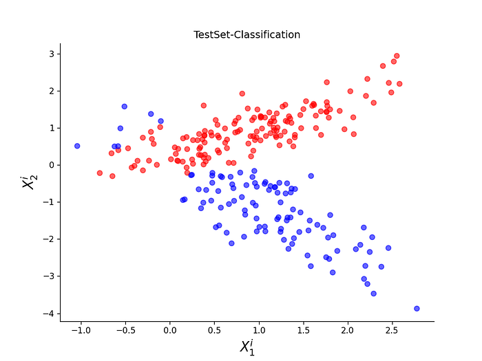
The ANN model is trained on the training-set by running an optimization algorithm (i.e., a Gradient Descent) which finds the best values for the weights of the ANN. We then apply the ANN model on these data points and obtain a classification label for each data point in the test set. The output of such classification can be seen in the figure 8.
Non-Linear Classification
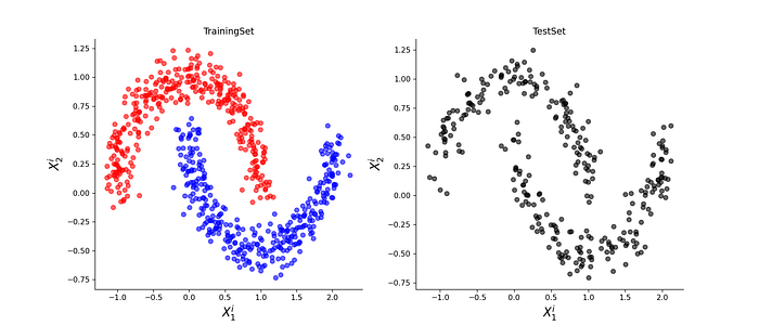
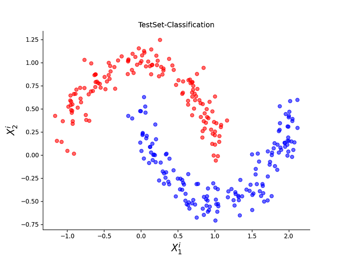
As it was mentioned earlier, a simple 3-Layer ANN is nothing but Linear Logistic Regression which means it can only classify linearly separable data. However, if we apply it to a data which is not linearly separable such as the one given in the figure 9 then it would fail miserably.
This means we must construct a network with multiple hidden layers. For this we modify the previous ANN and add two hidden layers with 5 Neurons in each layer as shown in the figure 10.
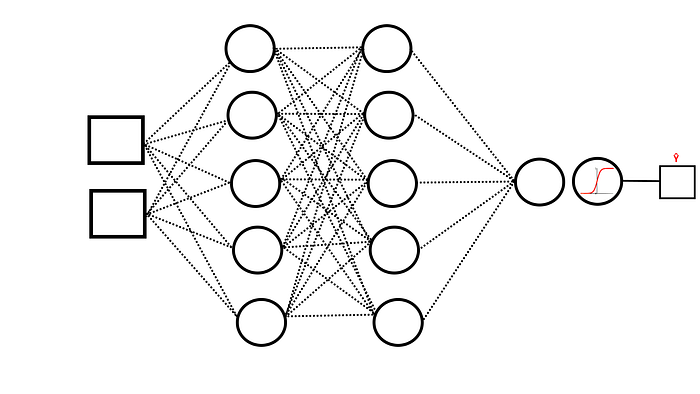
We apply this larger network on training set in figure 9 and obtain a set of optimized weights for this new network. Then we apply this network on the respective test-set and obtain the classification probabilities. The class labels can be obtained by applying a threshold on the probabilities (e.g., >0.7). The result of such network is shown in figure 11 below.
Final Remarks
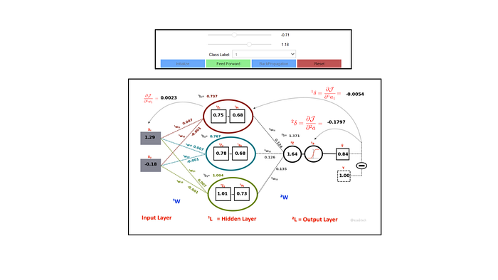
In this article, you have learned what are ANNs, how to formulate, and construct one from scratch in python. You have also learned how to apply ANNs for predicting class labels of both the linearly separable as well as for data which is not linearly separable. You can learn further by an interactive visualization tool that you could run in your Jupiter notebook and see how the weights are updated.
Code:
https://www.github.com/azad-academy/MLBasics-ANN
Become a Patreon Supporter:
https://www.patreon.com/azadacademy
Find me on Substack:
Follow Twitter for Updates: