
During multivariate time series analysis, data contains multiple data measured over time. To manage model performance, it is recommended to do feature extraction to make data points more compact for models.
Feature extraction is choosing only "Informative" features that capture vital information and underlying patterns in multivariate time series analysis. As time series data is data redundant, to enhance interpretability and make models less prone to overfitting, redundant data should be removed. Reduced dimensions of data allows faster processing of time series and can also be used to apply machine learning techniques for valuable prediction. For automatic feature extraction, various deep learning techniques can be leveraged and it might not need much manual feature extraction. The only challenge with automatic feature extraction is that it will be computationally heavy and a black box model which will cause challenges during the interpretation phase.
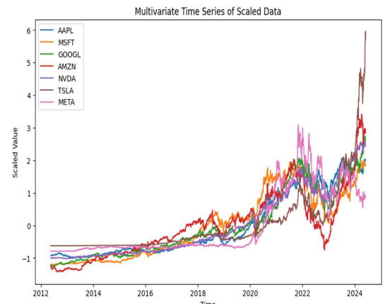
Multivariate time series refers to data with multiple interrelated points at a specific point in time. For analysis, magnificent seven stock data is taken from the yfinance library, and a sample time series without any feature engineering is demonstrated herby.
One of the key challenges with multivariate time series is that it has interdependence between variables. For example, the price of google stock might have a dependency on price of Apple or price of NVidia stock. As it is time time-based measurement, each stock will have a timestamp, and multivariate analysis emphasizes in capturing underlying relationship and pattern between such interdependence relationships.
Diagnosis
- Residual Plot
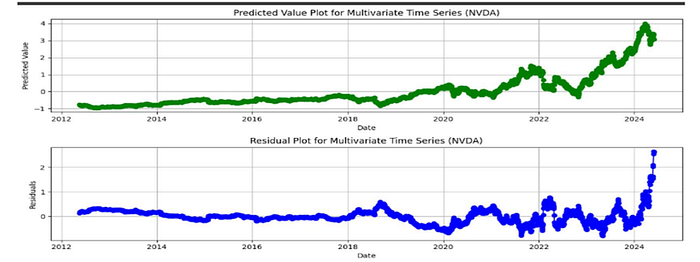
The plot shows the residual value over time along with the predicted value and there is huge difference in both the plot. This plot is being created using linear regression to get an idea about residuals. Residual eventually tells how much model is off from the actual value and helps in assessing model accuracy and identify errors. One of the first step of feature extractions starts with plotting residual plot and find any systematic error or pattern and hence improve model by using better features.
2. Correlation Heat Map
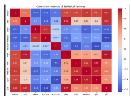
Another method to validate the need of feature engineering is correlation map. For statistical analysis not all the features might be required and correlation map helps in identifying how features are correlated with each other. By identifying correlation features, select the subset of features with most information and drop redundant feature. One of the empherical way of selecting feature is if the threshold is more than 0.7 (i.e 70%) then one of the similar feature should be selected rather than both the feature.
3. Machine Learning based Diagnostics
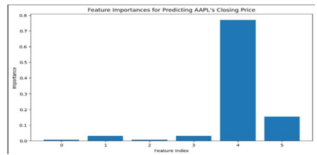
Early diagnosis of the redundancy or irrelevant data can help in making informed decisions about feature extraction. There are some challenges with a correlation heat map (linear relationship) and to overcome those challenges machine learning based model should be used to discover the value of features and remove features with lower weights.
Damages
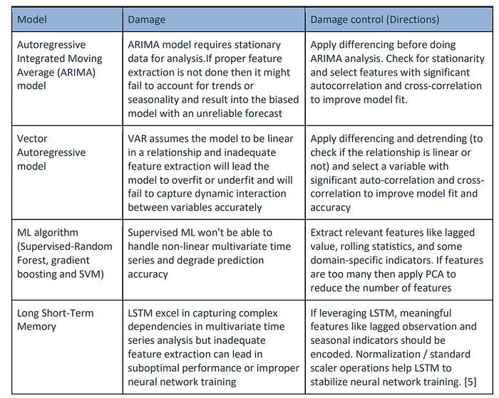
Directions
- Autocorrelation and Lag feature Extraction
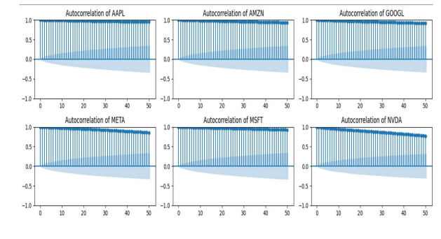
Autocorrelation: Autocorrelation refers to correlation of a variable with itself at different time lags and it helps in understanding how a variable is correlated with its own past value. From visual perspective significant spikes indicate potential time dependencies or pattern in the data. For feature engineering purpose 3 lags are used (1 day lag, 7 day lag and 30 day lag) to determine trends/seasonality or cyclical pattern.

For Feature extraction: There is no such lag which would be considered as best lag and hence a combination of lags must be considered to detect dependency within data. Interpretability of data is more important in feature extraction then high autocorrelation lag.
2. Differencing

Differencing is a technique used to transform data to remove trends and seasonality. Differencing involves subtracting a previous value from current value and can reduced the data but still maintain the pattern. Also, for models like ARIMA it improves stationarity. To check the need of differencing, first check if data has stationarity component within itself. To check stationarity, conduct Augmented Dickey Fuller Test (ADF TEST).
3. Cross-Correlation
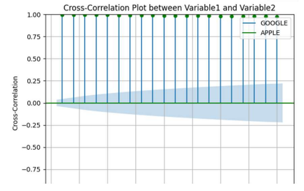
Cross-correlation is a powerful technique to understand lagged relationships between different variables. Unlike correlation which measures the overall linear relationship, cross correlation focuses on changes that are relative to another variable. By computing cross-correlation it helps to predict target value from target variable and another variable at different lag.
4. Time-Based Feature extraction
Rolling Mean:helps in highlighting underlying trends and it reduces overall noise
Rolling Standard Deviation: helps in highlighting volatility and it complements rolling mean
5. Shape based Feature extraction
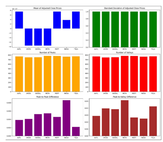
Peak and valley count captures the overall frequency of event and potentially indicates change in volatility level. Peak to peak difference is absolute difference between highest and lowest value and peak to valley difference is absolute difference between a peak and closest valley. This shape-based feature extraction are used to understand data characteristic for feature engineering along with it gives ideas about noise sensitivity and task specific relevance.
6. Principal Component Analysis
PCA helps in feature extraction by reducing dimension and capturing maximum variance within data.
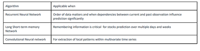
7. Automatic Feature Extraction (Neural Network)
—
Write me feedback on my article at parth.dave.ca@gmail.com