
Circular Convolution
First, let's recall what is a circular convolution. On the discrete sequences (e.g., vectors), circular convolution is the convolution of two discrete sequences of data, and it plays an important role in maximizing the efficiency of a certain kind of common filtering operation [1]. By definition, circular convolution can be formally described as follows.
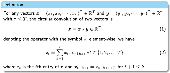
Here, the vector x is of length T, while the vector y is of length τ. If we follow the definition of circular convolution, then the resulting vector z is also of length T, just same as the vector x.
According to the definition of circular convolution, we can use some simple examples to help understand the concept:
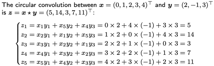
As can be seen, the circular convolution of two vectors essentially takes the linear system. It basically provides insight into building convolution matrix and circulant matrix.
Convolution Matrix
Following the above notations, if we have vectors x (of length T)and y (of length τ), then the circular convolution can be written as a system of linear equations:

To check how to build a convolution matrix by using the convolution operator, we utilize the following example:
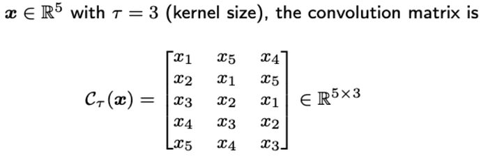
In this case, the convolution matrix has 5 rows (same as the length of x) and 3 columns (same as τ), and its columns are given by
- (x1, x2, x3, x4, x5) starting from x1 to x5;
- (x5, x1, x2, x3, x4) with the first entry as x5;
- (x4, x5, x1, x2, x3) with the first two entries as x4 and x5.
Then, the above-mentioned example now becomes
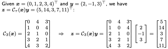
As can be seen, the result is same as the circular convolution.
Circulant Matrix
Recall that the convolution matrix works on the vector x of length T, is it possible to keep the vector x and build a certain kind of matrix on y?
The answer is yes! Let's check out an important property of circular convolution:
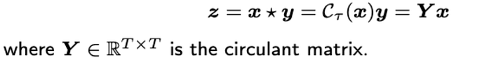
According to the definition of circular convolution, we can build a circulant matrix Y of size T-by-T on the vector y of length τ. Since τ is not greater than T, the circulant matrix Y is sometimes sparse. For example, we have
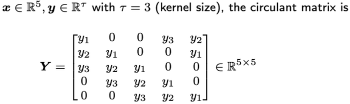
There are 5 columns in the circulant matrix. Note that the first column is (y1, y2, y3, 0, 0), in which the last two entries of the first column are filled with zeros.
Then, the above-mentioned example now becomes:
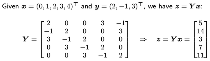
As can be seen, the result is same as the circular convolution.
Discrete Fourier Transform
Discrete Fourier transform (DFT) is an important concept in mathematics and has broad applications in the fields of digital signal process and image processing. The DFT is the most important discrete transform, used to perform Fourier analysis in many practical applications [2]. Since the implementation of DFT usually employ efficient fast Fourier transform (FFT) algorithms, the terms FFT and DFT are often used interchangeably [2].
Note that the FFT is an efficient algorithm for computing the DFT (see [3] for the difference between DFT and FFT). It is the name for any efficient algorithm that can compute the DFT in about O(n log n) time, instead of O(n^2) time [3].
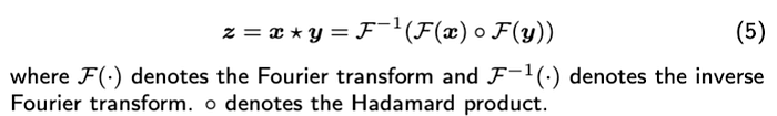
In this post, we can utilize the fact that: a convolution in the time domain is a product in the frequency domain. The DFT convolution theorem can be summarized as follows,
Then, the above-mentioned example now becomes:
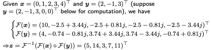
Here, the vector y is filled with zeros in the last two entries, and it is indeed the first column of the circulant matrix Y.
It is possible to use the NumPy package to compute the FFT and the inverse FFT.
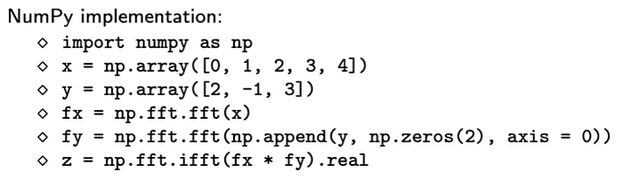
Notably, to perform Hadamard product, fx and fy should have the same length.
Conclusion
In signal processing, it can be shown that the convolution in the time domain is a product in the frequency domain. If one transforms vectors to the frequency domain, we can use the DFT (or FFT for realistic computation) to achieve fast computation, which is essentially the inverse FFT of the Hadamard product of transformed vectors. To reach the final property between circular convolution and DFT, we introduce some basic concepts: circular convolution, convolution matrix, and circulant matrix.
Thank you for reading this story!
References
[1] Circular convolution on Wikipedia: https://en.wikipedia.org/wiki/Circular_convolution
[2] Discrete Fourier transform on Wikipedia: https://en.wikipedia.org/wiki/Discrete_Fourier_transform
[3] What is the difference between the DFT and FFT? https://math.stackexchange.com/q/30464/738418