Decision tree is one of the simplest and easiest model to run. It is one of the simplest known model for solving classification and prediction problems. It is simple to learn and visualize too. And, to be frank, in simple words, it can be easily converted into rule based system. This is the reason, I termed it as one of the easiest to understand and make others understand too. For understanding of node calculation in this model using information gain method, you can definitely look into the below post:

Understanding for the calculation is good enough and always a gain to better understand code, lets code the same using python:

Decision Tree developed in Python

Import libraries

import pandas as pd
from sklearn.datasets import load_iris
from sklearn.model_selection import train_test_split
from sklearn.tree import DecisionTreeClassifier
from sklearn.metrics import accuracy_score, confusion_matrix

### Loading deafult iris data into variable

data = load_iris()

dir(data) # to check the attributes inside data output will be :

['DESCR',
 'data',
 'feature_names',
 'filename',
 'frame',
 'target',
 'target_names']

### Taking independent features and dependent features(target)

independentFeatures = data.data
dependentFeatures = data.target
predicted_class = data.target_names

### Split the dataset to train and test the model i.e, 80/20 Here train variables will be used for training the model and once training is done, test variables will be used for validating the trained model.

X_train, X_test, y_train, y_test = train_test_split(independentFeatures, dependentFeatures, test_size=0.20, random_state=42)

### Create Decision tree model and train

decisionTree = DecisionTreeClassifier(random_state=0)

### Predict using the trained model

y_pred = decisionTree.predict(X_test)

### Plotting confusion matrix with normalization and without normalization

from sklearn.metrics import plot_confusion_matrix
import matplotlib.pyplot as plt
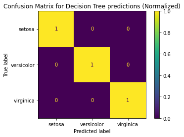
plot_confusion_matrix(decisionTree, X_test, y_test,display_labels = predicted_class, normalize = 'true')
plt.title("Confusion Matrix for Decision Tree predictions (Normalized)")
plt.show()

## Output of above plot will be :

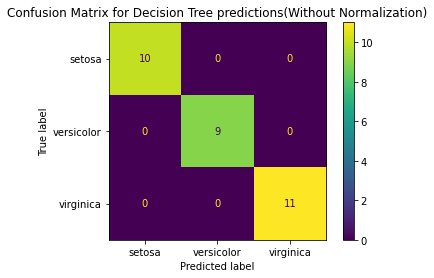
plot_confusion_matrix(decisionTree, X_test, y_test,display_labels = predicted_class, normalize = None)
plt.title("Confusion Matrix for Decision Tree predictions(Without Normalization)")
plt.show()

## Output of the above plot will be:

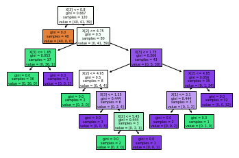
### If required you can plot the decision tree learnt by the model using below code

from sklearn.tree import plot_tree
plot_tree(decisionTree,filled=True)
plt.show()

Output of the above code will be:

Thats it, we are done with the code in python to develop decision tree. And, it is able to predict. In current example, it has very little data and there is no depth decided while training the model. It is predicting 100% accurate. But in actual environment, when independent feature will be more and complexity will be higher. We need to do data pre processing and then apply pruning, play with depth of the model to come over problems like overfitting and under-fitting.

For beginning, we are ready in few lines of python code and importing some of the libraries with our decision tree model.

For installing above libraries, use pip install <<libraryname>>. And, above code is written in python 3.X and above.

I mentioned about overfitting and underfitting. It is most common term in ML. And, Decision Tree model tends to overfit and under-fit very fast.

Complexity of model makes it Overfit and over simplicity or undertrained model comes under Under-fitting.

To Stop overfitting, we have to perform pruning and decides the depth of trees. How it works well to avoid overfit : Pruning is Data compression techinque and it means reducing down the features which are not adding any value to the tree. E.g, feature A and feature B provides same information gain to the data, then there is no point having both features while training the model. And, given a situation where number of features are too much and all are used to train the model, then you can understand how useful pruning will become to generalize and converge better.

And, similarly if our model is trained with all the features and it is not converging better with the new data. It means to generalize better we need to reduce down the features or depth of the tree and increase the train data size.

Advantages of DT is simple to understand and explain. Disadvantages is that it tends to overfit and underfit very fast. I hope we have touched the depth of DT and with the knowledge of node calculation and coding, we are ready to deal with actual rule based problems to be converted in model and work better. Happy Coding!