
SELECT *
FROM R, S, T
WHERE R.a = S.b AND S.c = T.d AND T.e = 10;
You're not telling the database:
"First, scan table T, then filter where T.e = 10, then join with S…"
Instead, you say what you want — all rows where those conditions hold true — and the database figures out the how internally.
That's why RDBMSs need this 3-step flow:
- Understand the query (Parsing & Validation)
- Decide the best way to execute it (Optimization)
- Run it efficiently (Execution)
Each stage transforms the query into a more concrete, machine-friendly form — from text → tree → executable plan → results.
Let's break this process down step-by-step and see why each part exists.

Step 1. Parsing and Validation
Purpose:
Convert the SQL text into a structure the database can work with — a logical query tree.
What Happens:
- Lexical analysis: breaks the SQL text into tokens (keywords, identifiers, etc.).e.g.,
SELECT,FROM,R,WHERE, etc. - Syntax analysis (parsing): checks grammar — ensures it follows SQL rules.
- Semantic validation: ensures the query makes sense:
- Tables
R,S, andTexist. - Columns
a,b,c,d,ebelong to them. - Data types are compatible for comparisons.
If all checks pass , the system creates a logical query tree —
a tree structure representing the relational operations (SELECT, JOIN, FILTER) needed to answer the query.
Step 2. Query Optimization
Purpose:
Find the most efficient way to execute the query.
There are many possible ways to get the same result — but they vary a lot in speed.
Example:
SELECT *
FROM Customers, Orders
WHERE Customers.id = Orders.customer_id;
Possible strategies:
- Scan
Customersfirst, thenOrders. - Or scan
Ordersfirst, thenCustomers. - Use indexes if available.
The optimizer estimates the cost (time, memory, CPU, disk I/O) of each plan and picks the cheapest one.
It transforms the logical query tree into a physical execution plan — where each node represents a concrete action:
Step 3. Query Execution — How the Engine Actually Runs the Plan
Once the optimizer picks the best plan, the query execution engine takes over. This is where the database does the work — reading data, joining tables, sorting results, and producing the final output you see.
Think of the execution plan as a tree of physical operators, where each operator performs a specific task:
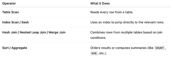
Each of these operators is like a small worker — it knows how to do one job well, and it can call other workers below it in the plan tree to get the data it needs.
The Iterator (Pull) Model
Most databases use what's called the iterator model (or pull model) for query execution.
Here's how it works: Each operator implements three methods:
Open()     # initialize state
GetNext()  # fetch next row or batch of rows
Close() # clean up- The top operator (for example, a
Join) doesn't "push" data up. Instead, it pulls data from the operators below it by callingGetNext(). - Each operator calls
GetNext()on its own child operator — creating a chain of calls from the top of the tree down to the data on disk.
Here's a simplified flow:
          Nested Loop Join
                ▲
                │  calls GetNext()
           Hash Join
     ▲                 ▲
     │                 │
 Table Scan(S)   Table Scan(T)
So when the user runs SELECT ..., the top operator keeps asking its children for the next rows until there's no more data to pull.
This "row-by-row" pulling is simple and modular — databases can easily add new operator types using the same interface.
That's why this design has lasted for decades — it's elegant and extensible.
Vectorization — Making It Fast for Modern CPUs
The iterator model is flexible but not very fast:
Each GetNext() call handles one row at a time, which causes:
- A lot of function calls.
- Poor CPU cache locality.
- Wasted potential of modern CPUs that can process multiple values at once (SIMD).
To fix this, databases introduced vectorized execution.
Instead of returning a single row, each GetNext() now returns a batch (for example, 1,000 rows).
The CPU can then process these in chunks using SIMD (Single Instruction, Multiple Data) — one operation applied to multiple values simultaneously.
Combine that with columnar storage (where data from the same column is stored together in memory), and you get a massive performance boost — perfect for analytics and decision-support queries.
Code Generation — The Final Optimization Layer
Some modern engines take it one step further. Instead of interpreting the plan operator by operator, they generate optimized machine code tailored to your query.
- The database translates the execution plan into C or LLVM code.
- The code is compiled at runtime and executed directly on the CPU.
- This eliminates the overhead of function calls and interpretation loops.
It's like turning your SQL query into a custom-compiled program — lightning-fast, specialized, and efficient.
Systems such as HyPer, MonetDB, and modern versions of PostgreSQL, DuckDB, and Snowflake use these techniques to get near "native" performance.