Wrangling through Dataland

The feature richness of the Ames housing dataset (2011) is both alluring and bewildering in equal measure. It is easy to become entagled in its bountiful features while trying to uncover its patterns. It is first and foremost useful to understand that the Ames dataset fits into the long-established hedonic pricing method to analyzing housing prices. Some domain knowledge will go a long way.

I had previously studied statistics/econometrics in some detail. Cognizant of the "big data" revolution and intrigued by its promise, I have immersed myself in coding and machine learning these past few months. It was in this process that I encountered the Ames housing dataset. I approached it with a combination of traditional econometric research and machine learning tools.

I chose to stick to transparent linear models where the goals of both prediction and statistical inference may be pursued together. This meant running ordinary least squares (OLS), Ridge and Lasso regression models. Please note that the analysis I undertook was on the full original Ames dataset, and not the Kaggle version of the dataset.

Hedonic Pricing Method

In econometric research, one attempts to expand research horizons by standing on the shoulders of previous researchers in the subject matter. No two houses are exactly identical, and the basic idea of hedonic price modeling is that neighborhood-specific and unit-specific characteristics help determine house prices.

It is therefore useful to regurgitate the usual suspects affecting house prices. If the dependent (or target) variable is the sale price, then naturally the larger the house the higher the price, all else being equal. That should be as self-evident as asserting that an 18-inch pizza will probably cost more than a 12-inch pizza. So property size measures will be key variables, and there are several such variables in the Ames dataset. A more interesting question might be how and why the price per square foot might differ from house to house, which is like asking why certain pizzerias are able to charge a higher price per slice. Real estate professionals too tend to focus on price per square foot (or meter) instead of the overall price. But that is not the goal in this article.

Any home buyer would have heard of the expression "location, location, location", which also happens to be the title of a popular British TV show on house buyers that has been on air for 19 consecutive years. So one would expect neighborhood "location" and associated characteristics, such as access to amenities (e.g. good schools, leisure facilities), transport networks (e.g. near a metro station), neighborhood aesthetics (e.g. tree-lined streets, handsome houses), and socioeconomic prestige among others, to have an impact on house prices.

Another group of factors commonly said to be important for determining housing prices is the number of rooms, particularly bedrooms and bathrooms, and the condition of the kitchen. Beyond this, the age and physical condition of the house are also important, as are the construction materials and any structural improvements to the property.

The factors that effect housing prices may be summarized as property size, location desirability, nearby amenities, number of rooms, construction materials, and age and condition of the structure. Armed with this prior research, I took to analyzing the data using Python.

Data Cleaning & Outliers

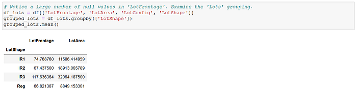
The first task was data cleaning, as ever. The dataset had 2,930 observations initially, and I immediately dropped three variables that had less than 300 observations each. The "LotFrontage" (linear feet of street connected to property) variable, which I thought could be important, was missing 490 observations. I filled the missing values with the average "LotFrontage" when grouped by their respective "LotShape" categories.

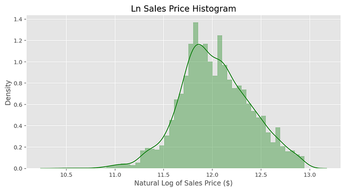
I then rendered a histogram of the dependent variable, "SalePrice". It was immediately obvious that it had extreme high values (a long right-tail) and was not distributed normally. This suggested that the data contained a lot of outliers. Dealing with outliers can be tricky in that some of them may provide important information, so one doesn't want to define outliers too liberally and then chuck them all out.

Given the importance of property size metrics, I quickly zoomed in on "GrLivArea", "LotSize" and "GarageArea" as potential explanatory variables. It is uncommon in the US to include the basement square footage in the measure of a property's size. In fact, Fannie Mae and ANSI guidelines forbid the counting of basement square footage in appraising a property's living area, though one can imagine that it is still likely to exert some impact on property prices. I consequently chose to separate the basement size measure, and constructed a finished basement area variable, "BaseLivArea", from other basement measures.

It was now time to search for outliers. I looked for those observations in "SalePrice", "GrLivArea" and "BaseLivArea" respectively that were either under or above 3 standard deviations away from their respective mean values. There were no observations in the "under" category, but there were 66 observations in the "above" category across all three variables. I deleted these 66 observations, which comprised approximately 2.3% of the sample, from the analysis.

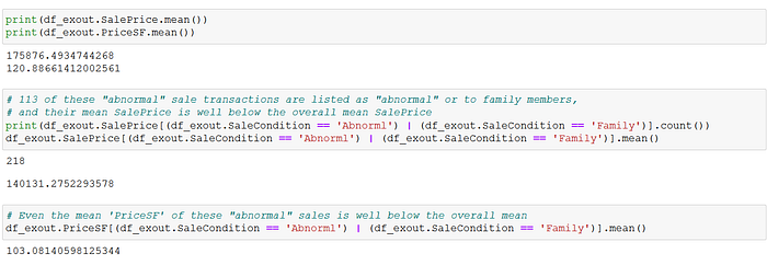
Then, I looked into the "SaleCondition" variable, which recorded the type of sales for each transaction, Most observations were in the "Normal" sale category, but there were 218 observations recorded as either "Abnormal" or "Family" (intra-family sale). I zoomed in on these, and noted that both their mean and median sale prices (and price per square foot) were well below those of the overall sample. This prompted me to exclude these 218 unusual sale transactions from the analysis. If these transactions were not primarily commercial in nature, then their inclusion in the dataset would introduce bias into a model trying to estimate the economic relationship between housing characteristics and house prices.

Feature Engineering

I had now reduced the number of observations from the original 2,930 to 2,617. I then constructed a variable to express the age of the property, "Age", before undertaking a natural log-transformation of "SalePrice" . The histogram of log sale prices definitely appeared more symmetrical, with less extreme values. The resulting model is a log-linear model, meaning a log dependent variable with linear explanatory variables.

The next problem was the dearth of a location desirability variable. There were 28 neighborhoods listed in the "Neighborhood" variable, but it's unclear how to rank them. It might be obvious to rank these neighborhoods by their price per square foot, and use this as a location desirability measure, but this artificial construct would naturally be correlated to the house price. That's just not good research methodology because one would be constructing a composite feature variable created partly from the target variable itself. An obvious proxy for location desirability would be to rank each neighborhood by its average household income, but the dataset did not have such data available.

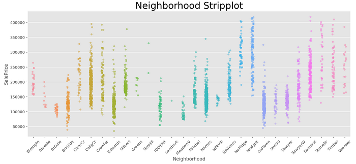
A simplistic way to deal with this would be to dummify these 28 neighborhoods and chuck them all into the model. The problems with having individual dummies for such a large number of neighborhoods are:

1. There are only a handful of observations for some neighborhoods, with less than 30 observations for eight of them, and less than 100 for the majority of them out of 2,617 sample observations;
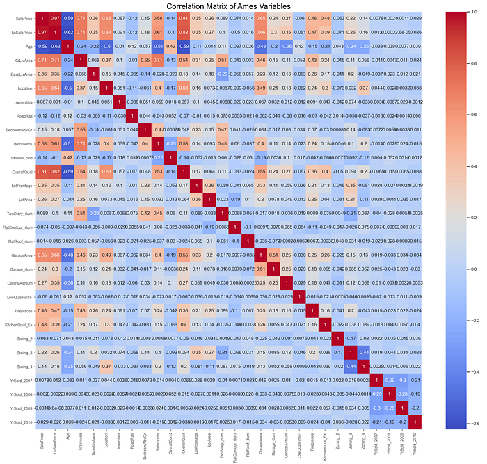
2. There would be significant multicollinearity between certain neighborhoods that share similar characteristics and therefore have similar distribution of house prices, as may be observed in the stripplot above; and
3. If one had any interest in statistical inference, then one cannot draw much inference from such dummies without first having some prior knowledge of how these neighborhoods might rank in terms of desirability.

I chose instead to construct an ordinal neighborhood "Location" desirability variable out of various building quality and condition variables in the dataset, notably "OverallQual", "OverallCond", "ExterQual", "ExterCond" and "Functional". The motivation behind my methodology was the assumption that the more desirable a neighborhood, the better the quality of its housing structures and their condition.

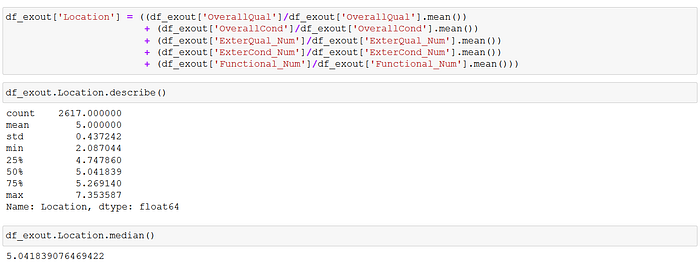
With no additional information or insight, I decided that it was best to keep things simple and just allocate 4 ordinal values for "Location" desirability: 1 (low), 2 (mid-low), 3 (mid-high) and 4 (high). The 28 neighborhoods were sorted by their mean "Location" scores, and I used the overall "Location" mean value to divide the neighborhoods into lower- and upper-half groupings.

The mean "Location" value conveniently split the 28 neighbourhoods into 14 neighborhoods at or above it, and 14 below it. These two groups were then halved again, so that the seven neighborhoods with the lowest mean "Location" scores were assigned "Location"=1, the subsequent seven neighborhoods were assigned "Location"=2, the next seven were assigned "Location"=3, and the remaining seven were placed in "Location"=4.

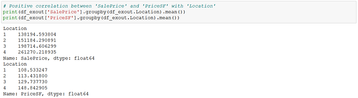
Following these assignments, I checked the mean and median "SalePrice" and price per square foot of each "Location" rank, and there was a clear positive correlation between the "Location" score and both price variables. This verified that the "Location" variable as constructed could be a good proxy for neighborhood desirability.

That was the most work with a single variable in the exercise. I also created year dummies because the data straddled the 2008 financial crisis, which had a major impact on US housing prices. Moreover, I created four dummies for each of the four zones ("Zoning"), one dummy for being near an artery road or railway line ("RoadRail"), one dummy being near positive amenities such as a park ("Amenities"), one for garages ("Garage"), one for flat roofs ("FlatRoof"), one for houses higher than one floor ("TwoStorey"), and one for a flat contour of the property lot ("FlatContour").

In terms of indoor unit-specific features (other than the size variables), I picked "OverallQual" as an ordinal variable, "OverallCond" as an ordinal variable, "Bedrooms" for number of bedrooms, "Bathrooms" for number of bathrooms, "Fireplaces" for number of fireplaces, "CentralAirCond" as a dummy with 1 for having central air conditioning, and "ExcellentKitchen" as a dummy with 1 for a kitchen rated as "excellent".

It is commonly said that "the kitchen sells the house", and that fireplaces are particularly desirable. So we shall see.

Regression Analysis

The correlation matrix of the resultant engineered data showed that the correlations among the chosen explanatory variables were generally under +/-0.50. The only explanatory variable pair that exhibited correlations greater than +/-0.70 was the "GrLivArea-Bathrooms" pair. "Bathrooms" also showed elevated correlations (over 0.50) with "Age" and "OverallQual" separately. I consequently decided to drop the "Bathrooms" variable from the regression modeling to reduce multicollinearity.

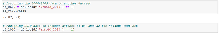
The engineered data was split before running the regression analyses. The 2010 sales data were reserved as the holdout test set, while the 2006–2009 data were used for the train-validation process.

The regression model incorporated the following explanatory variables: Age, GrLivArea, BaseLivArea, LowQualFinSF, GarageArea, LotArea, LotFrontage, Location, Bedrooms, Fireplaces, OverallQual, OverallCond, Amenities (dummy), RoadRail (dummy), TwoStorey (dummy), FlatContour (dummy), FlatRoof (dummy), Garage (dummy), CentralAirCond (dummy), ExcellentKitchen (dummy), Zoning_2 (dummy), Zoning_3 (dummy), Zoning_4 (dummy), and the year dummies.

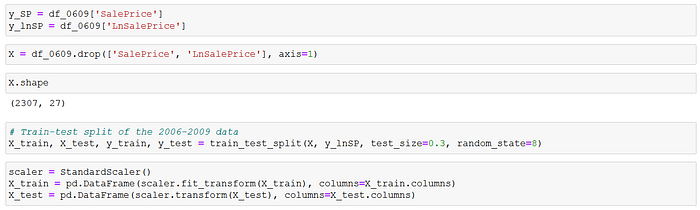
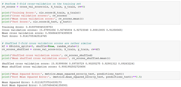
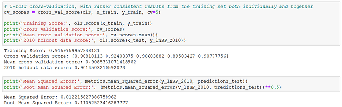
The target variable was the natural log of "SalePrice". I used an 70–30 train-validation split for the 2006–2009 data. The explanatory variables were also standardized before running the regressions. The train-validation set was subsequently run through the OLS, Ridge and Lasso linear regression models. All three linear models provided train-test scores of 0.91–0.92, MSE of approximately 0.011, and RMSE of approximately 0.106.

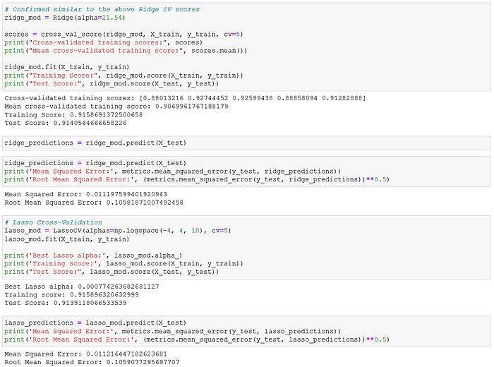
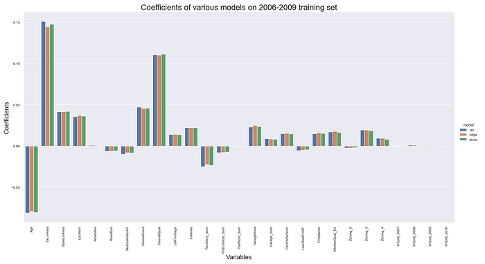
Thus, all three linear models produced rather consistent scores. The coefficients were also rather consistent across the models, as may be observed below. These results suggested very stable model parameter estimates. The model coefficients imply that the six largest effects on house prices in Ames were (in descending order) the above ground living space (positive), overall quality (positive), house age (negative), overall condition (positive), basement living space (positive) and location ranking (positive). These six variables were all also statistically significant at the 95% level, as I will discuss below.

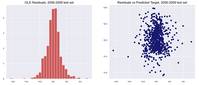
Ordinary least squares regression assumes that the residual errors are independent of each other with a normal distribution, mean zero and homoskedastic. The skew and kurtosis indicated that the error distributions were approximately normal with mean zero. The residual plots also indicated that the various OLS assumptions regarding the distribution of the residuals may be assumed to hold. The full residual analysis is available at my GitHub page with the link at the bottom of the article.

Holdout Test Scores

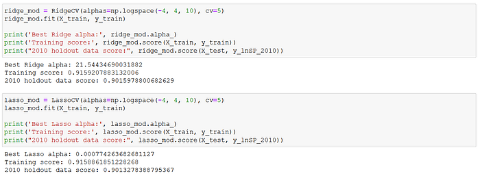
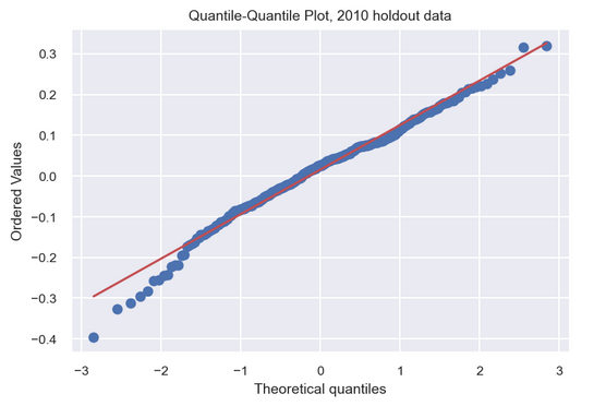
For the moment of truth, I tested the model on the 2010 holdout data. There was a slight drop in the R-squared for the 2010 holdout test set from the training (full 2006–2009) data (0.9014 versus 0.9160), but the scores were again rather consistent across the OLS, Ridge and Lasso models. The OLS regression's MSE and RMSE scores were 0.012 and 0.110 respectively on the holdout test set, again showing a slight drop from the train-validation results above.

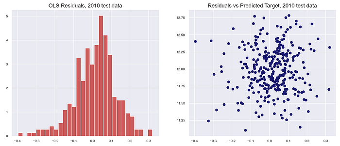
The residuals were also approximately normally distributed with mean zero. The quantile-quantile plot (qq-plot) of the test residuals in particular indicated a reasonable fit to a normal distribution.

Statistical Inference

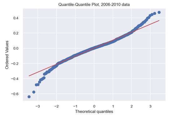
I utilized the full 2006–2010 dataset for statistical inference. This is one of the key differences between running a regression model for prediction purposes and doing it for causal inference. When we train a model for prediction, we split the data and segregate a test set to evaluate the accuracy of the model predictions (as executed above). In statistical inference, on the other hand, the full dataset is typically used to derive the parameter estimates, which are evaluated against various test statistics.

The qq-plot for the model incorporating the full 2006–2010 dataset cautions against an overly optimistic use of the model to predict house prices. The qq-plot indicates that the model tends to under-predict house prices in the highest quantile and over-predict those in the lowest quantile. So while the final model may explain over 91% (R-squared) of the variation in house prices, it is not reliable when dealing with houses at the extremes of the price range. The model is most effective when targeting those properties with prices in the 25%-75% inter-quartile range.

As for calculating exactly how the various explanatory variables might affect house prices, I would first need to compute the individual coefficient standard errors and p-values to determine if a particular variable is statistically significant. I would also need to revert back to the original unstandardized explanatory variables. The resulting summary table of the OLS regression results on the full 2006–2010 data is below, from the Statsmodels module.

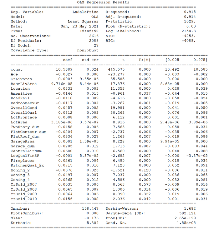
As may be observed, the overwhelming majority of the explanatory variables in the OLS model are statistically significant at the 95% level (i.e. p-value < 5%), as indicated by the individual t-statistics and associated p-values. The exceptions are the "RoadRail" and "LowQualFinSF" variables. The six variables found to have the largest impact on the house sale price are all statistically significant, as mentioned above.

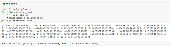
As a reminder, the model is log-linear where the target variable is the natural log of "SalePrice". To compute the impact of a unit change in each variable on the "SalePrice", we would first need the exponent of each coefficient. Moreover, the coefficients of a log-linear model imply the percentage change in the target variable for small unit changes in the explanatory variable. To get the specific dollar impact, it is best to use the mean "SalePrice" as the reference comparison.

The dollar impact of a one-unit change in each explanatory variable on the average house price in Ames is listed in the table on the left. To keep it brief, I will only discuss some of those variables found to be statistically significant.

For example, an increase in the "Age" of the housing unit by one year will reduce the average house price by $487, all else being equal. A one-category increase in the "Location" (remember that this was a four-category ordinal variable) by comparison will raise the average house price by $6,050 (the fourth variable), all else being equal.

Moreover, a fireplace will add $4,725 to the average house price, while a kitchen rated "excellent" will bump up the price by $13,250 (the 19th and 20th variables).

So indeed "the kitchen sells the house"!

Conclusion

Based on insights from the hedonic pricing literature on house prices, I zoomed in on various property size measures as likely important features for the regression model. I also undertook a log transformation of the highly skewed house price target variable.

There followed extensive feature engineering on various structural and internal factors expected to be significant determinants of house prices, principally a location desirability variable, zoning dummies, build quality and condition, proximity to amenities, and a highly-rated kitchen among others. The engineered data was then run through three linear regression models: OLS, Ridge and Lasso.

Stable results and scores were found across the three linear models. The OLS regression coefficients nearly matched those derived from the Ridge and Lasso regressions. The modeling achieved an R-squared of approximately 91-92% on the training-validation sets, and this was consistent across the OLS, Ridge and Lasso regressions. It subsequently managed to secure a 90% score on the 2010 holdout test set, along with MSE and RMSE scores of 0.012 and 0.110 respectively. The results were again consistent across the various algorithms.

The assorted property size variables, namely internal living area, basement finished area, lot area and garage area, were all found to be positively correlated to the sale price and statistically significant. Build quality and condition were also found to be among the most important determinants of house prices, as was location desirability.

There was no need for any abstruse black-box algorithm to achieve these results. Just straight-up linear regression that is transparent and interpretable, and where the individual explanatory variables may be subjected to hypothesis testing. Thus, the goals of prediction and statistical inference could be pursued together. More importantly, the linear regression results can be easily communicated to lay audiences, at both the model and individual variable levels.

(The full Python code and data for this exercise are available in my GitHub repository. If it is problematic rendering the GitHub notebook files directly, use nbviewer.)

If you saw value in reading articles like this, you may subscribe to Medium here to read other articles by me and countless other writers. Thank you.