Fourier Transform is a powerful way to view data from a completely different perspective: From the time-domain to the frequency-domain. But this powerful operation looks scary with its math equations.

Transform time-domain wave to frequency-domain:

The image below is a good one to illustrate the Fourier Transform: decomposite a complex wave into many regular sinusoids.

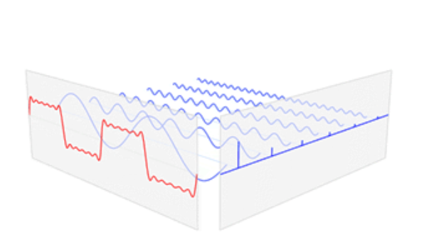
Here is the complete animation explains what happens when transforming the time-domain wave data to frequency-domain view.

We can easily manipulate data in the frequency domain, for example: removing noise waves. After that, we can use this inverse equation to transform the frequency-domain data back to time-domain wave:

Let's temporarily ignore the complexity of FT equations. Pretend that we have completely understood the meaning of the math equations and let's go use Fourier Transform to do some real work in Python.

The best way to understand anything is by using it, like the best way to learn swimming is getting wet by diving into the water.

Mix clean data with noise

Create two sine waves and merge them into one sine wave, then purposefully contaminate the clean wave with data generated from np.random.randn(len(t)).

import numpy as np
import matplotlib.pyplot as plt
plt.rcParams['figure.figsize'] = [16,10]
plt.rcParams.update({'font.size':18})
#Create a simple signal with two frequencies
data_step   = 0.001
t           = np.arange(start=0,stop=1,step=data_step)
f_clean     = np.sin(2*np.pi*50*t) + np.sin(2*np.pi*120*t)
f_noise     = f_clean + 2.5*np.random.randn(len(t))
plt.plot(t,f_noise,color='c',Linewidth=1.5,label='Noisy')
plt.plot(t,f_clean,color='k',Linewidth=2,label='Clean')
plt.legend()

(Combining two signals to form a third signal is also called convolution or signal convolution. This is another interesting topic and nowadays intensively used in Neural Network Models)

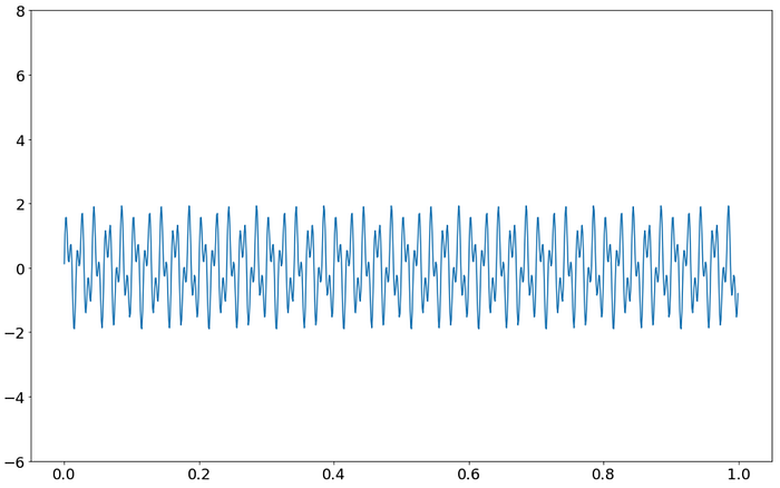
We have the waves with noise, black is the wave we want, green lines are noise.

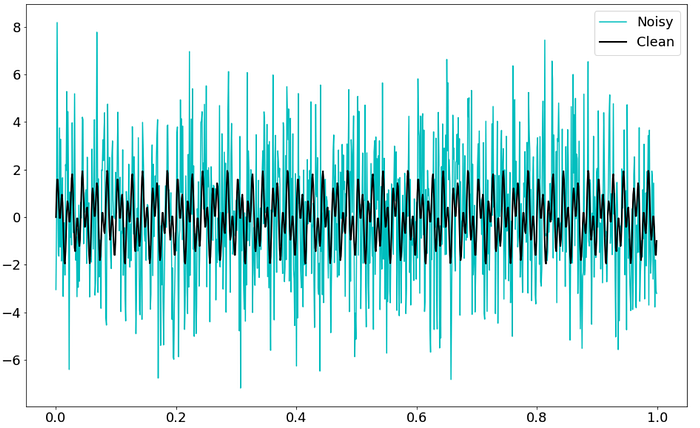
If I hide the colors in the chart, we can barely separate the noise out of the clean data. Fourier Transform can help here, all we need to do is transform the data to another perspective, from the time view(x-axis) to the frequency view(the x-axis will be the wave frequencies).

Transform from Time-Domain to Frequency-Domain

You can use numpy.fft or scipy.fft. I found scipy.fft is pretty handy and fully functional. Here I will use scipy.fft in this article, but it is your choice if you want to use other modules, or you can even build one of your own(see the code later) based on the formula that I presented in the beginning.

from scipy.fft import rfft,rfftfreq
n    = len(t)
yf   = rfft(f_noise)
xf   = rfftfreq(n,data_step)
plt.plot(xf,np.abs(yf))

• In the code, I use rfft instead of fft. the r means to reduce(I think) so that only positive frequencies will be computed. All negative mirrored frequencies will be omitted. and it is also faster. see more discussion here.
• The yf result from the rfft function is a complex number, in form like a+bj. the np.abs() function will calculate √(a² + b²) for complex numbers.

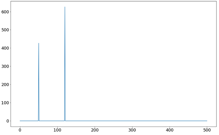
Here comes the magical Frequency-Domain view of our original waves. the x-axis represents frequencies.

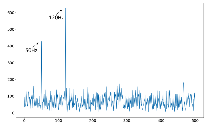
Something that looks complicated in the time-domain now is transformed to be very simple frequency-domain data. The two peaks represent the frequency of our two sine waves. One wave is 50Hz, another is 120Hz. Take another look back on the code that generates the sine waves.

f_clean     = np.sin(2*np.pi*50*t) + np.sin(2*np.pi*120*t)

Other frequencies are noises, which will be easily removed in the next step.

Remove the noise frequencies

With help of Numpy, we can easily set those frequencies data as 0 except 50Hz and 120Hz.

yf_abs      = np.abs(yf) 
indices     = yf_abs>300   # filter out those value under 300
yf_clean    = indices * yf # noise frequency will be set to 0
plt.plot(xf,np.abs(yf_clean))

Now, all noises are removed.

Inverse back to Time-Domain data

The code:

from scipy.fft import irfft
new_f_clean = irfft(yf_clean)
plt.plot(t,new_f_clean)
plt.ylim(-6,8)

As the result shows, all noise waves are removed.

How the transforming works

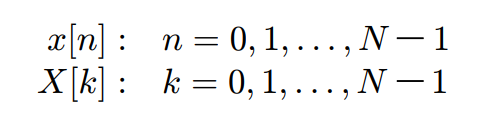
Back to the transform equation:

The original time-domain signal is represented by lower case x. x[n] means the time-domain data point in the n position(time). The data point in frequency-domain is represented by upper case X. X[k] means the value at the frequency of k.

Say, we have 10 data points.

x = np.random.random(10)

The N should be 10, so, the range of n is 0 to 9, 10 data points. The k represents the frequency #, its range is 0 to 9, why? the extreme condition will be each data point represent an independent sine wave.

In a traditional programming language, it will need two for loops, one loop for k, another for the n. In Python, you can vectorize the operation with 0 explicit for loops (Expressive Python).

And Python's native support of complex numbers is awesome. let build the Fourier Transform function.

import numpy as np
from scipy.fft import fft
def DFT_slow(x):
    x = np.asarray(x, dtype=float)# ensure the data type
    N = x.shape[0]                # get the x array length
    n = np.arange(N)              # 1d array
    k = n.reshape((N, 1))       # 2d array, 10 x 1, aka column array
    M = np.exp(-2j * np.pi * k * n / N)
    return np.dot(M, x)       # [a,b] . [c,d] = ac + bd, it is a sum
x = np.random.random(1024)
np.allclose(DFT_slow(x), fft(x))

This function is relatively slow compare with the one from numpy or scipy, but good enough for understanding how FFT function works. For faster implementation, read Jake's Understanding the FFT Algorithm.

Further thoughts — not a summary

The idea presented from Fourier Transform is so profound. It reminds me the world may not be what you see, the life you live on may have a completely different new face that can only be seen with a kind of transform, say Fourier Transform.

You can not only transform the sound data, but also image, video, electromagnetic waves, or even stock trading data (Kondratiev wave).

Fourier Transform can also be interpreted with wave generation circles.

The big circle is our country, our era. We as an individual is the small tiny inner circle. Without the big circle that drives everything, we are really can't do too much.

The Industrial Revolution happened in England rather than in other countries not simply because of the adoption of steam engines, but so many other reasons. — Why England Industrialized First. it is the big circle that only exists in England at that time.

If you are rich or very successful sometimes, somewhere, it is probably not all because of your own merit, but largely because of your country, people around you, or the good company you work with. Without those big circles that drive you forward, you may not able to achieve what you have now.

The more I know about Fourier Transform, the more I am amazed by Joseph Fourier that he came up with this unbelievable equation in 1822. He could never know that his work is now used everywhere in the 21st century.

Appendix — Four kinds of Fourier Transform

All Fourier Transform mentioned in this article is referring to Discrete Fourier Transform.

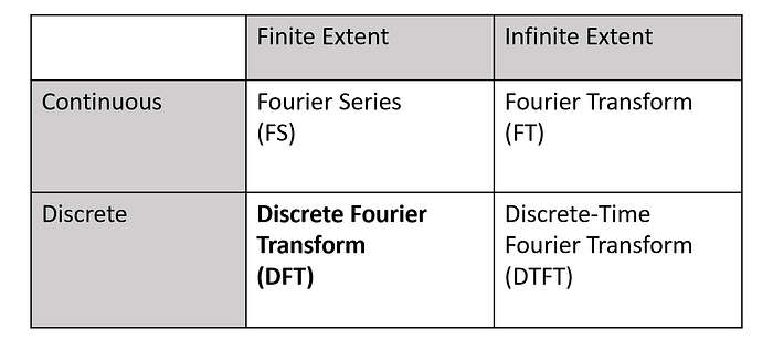
When you sit down in front of a computer and trying to do something with Fourier Transform, you will only use DFT - the Transform that is being discussed in this article. If you decide to sink your neck into the math swamp, here are two recommended books to read:

1. Frequency Domain and Fourier Transforms. Paul W. Cuff's textbook from Princeton.

2. Chapter 8 of the book Digital Signal Processing — by Steven W.Smith they provided the online link: DSP Ch8

References

1. An Interactive Guide To The Fourier Transform: https://betterexplained.com/articles/an-interactive-guide-to-the-fourier-transform/
2. Fourier Transforms With scipy.fft: Python Signal Processing:https://realpython.com/python-scipy-fft/
3. Understanding the FFT Algorithm:http://jakevdp.github.io/blog/2013/08/28/understanding-the-fft/
4. Frequency Domain and Fourier Transforms: https://www.princeton.edu/~cuff/ele201/kulkarni_text/frequency.pdf
5. Denoising Data with FFT [Python]: https://www.youtube.com/watch?v=s2K1JfNR7Sc&ab_channel=SteveBrunton
6. The FFT Algorithm — Simple Step by Step: https://www.youtube.com/watch?v=htCj9exbGo0&ab_channel=SimonXu

If you have any questions, leave a comment and I will do my best to answer, If you spot an error or mistake, don't hesitate to mark them out. Your reading and support is the big circle that drives me to keep writing more. Thank You.