In the previous article, we imputed missing values and removed outliers from the dataset with an isolation forest algorithm. This next article will showcase how we apply these two techniques to the training and test set. Afterwards, we will perform the pre-processing with scikit-learn on the data and train a Random Forest Regressor on the training data. The dataset used is the California Housing dataset, which can be downloaded on Kaggle or extracted from the GitHub-Repository. The pipeline, code, and inputs in this article are inspired and sometimes copied from the book "Hands-On Machine Learning with Scikit-Learn, Keras, and TensorFlow".

Pipeline

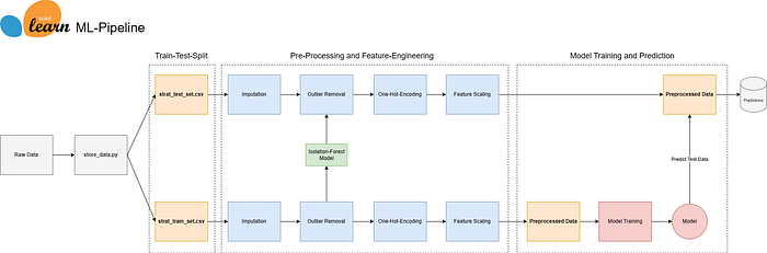
To recap from the previous article you find below the pipeline. So far the data has been split into a training- and test dataset. Missing values have been imputed and the outliers removed. Now it is time to further preprocess the data with a scikit-learn pipeline to one-hot-encode categorical variable and scale the features. Then we will apply a Random Forest Regressor using grid-search and cross-validation to obtain a suitable model.

Pre-Processing

The goal is to prepare the data for a regression problem using a pre-processing pipeline. First, the function creates a copy of the data and separates the target variable, which, in this case, is the "median house value". The target variable will be used later for training the model. Three new variables are created for different types of features: one for categorical features, one for features to be standardized using StandardScaler, and the last one for features to be scaled using MinMaxScaler.

Standardization (Standard-Scaler):

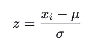
The standard scaler is standardizing the feature by taking each observation (xi), subtracting the mean, and dividing by the standard deviation. StandardScaler follows the standard normal distribution. Therefore, it makes mean = 0 and scales the data to unit variance.

Min-Max Scaler

MinMaxScaler scales all the data features in the range [0, 1] or else in the range [-1, 1] if there are negative values in the dataset.

The categorical variable is one hot encoded. For each category one new column will be made and if an observation falls in a particular category, a value of 1 is present otherwise the value 0 is present. See the code below for the implementation:

import os
import pandas as pd
import numpy as np
import joblib

from sklearn.compose import ColumnTransformer
from sklearn.pipeline import Pipeline
from sklearn.ensemble import RandomForestRegressor 
from sklearn.preprocessing import OneHotEncoder, StandardScaler, MinMaxScaler
from sklearn.model_selection import GridSearchCV, KFold

# Folder for Regression Model
FOLDER_REG = os.path.join(os.path.dirname(os.path.dirname(os.path.dirname(__file__))), "models", "california_housing_regression")


def data_preprocessing(data):
    
    # Create a copy of the data
    data_copy = data.copy()
    data_copy = data_copy.drop('median_house_value', axis=1)

    # Define numerical and categorical columns
    categorical_columns = ["ocean_proximity"]
    numerical_columns_standard = ["longitude", "latitude"]
    numerical_columns_minmax = [col for col in data_copy.columns if col not in categorical_columns + numerical_columns_standard]

    # Pipeline for categorical features
    cat_pipeline = Pipeline(steps=[
        ('one-hot-encoding', OneHotEncoder(handle_unknown='ignore')),
    ])

    # Pipeline for standard numerical features
    num_pipeline_standard = Pipeline(steps=[
        ('scale', StandardScaler())
    ])

    # Pipeline for minmax numerical features
    num_pipeline_minmax = Pipeline(steps=[
        ('scale min max', MinMaxScaler())
    ])

    # Create column transformer
    col_trans = ColumnTransformer(transformers=[
        ('cat_pipeline', cat_pipeline, categorical_columns),
        ('num_pipeline_standard', num_pipeline_standard, numerical_columns_standard),
        ('num_pipeline_minmax', num_pipeline_minmax, numerical_columns_minmax)
    ],
        remainder='drop',
        n_jobs=-1)
    
    # Fit and transform the data
    transformed_data = col_trans.fit_transform(data_copy)

    # Get the column names after transformation
    transformed_column_names = col_trans.get_feature_names_out()

    # Return both the transformed data and the column names
    return transformed_data, transformed_column_names

The transformation is then applied with a Column-Transformer to handle the different columns accordingly. The function will return the transformed data in a numpy-array as well as the column names which are of later usage to assess the feature importance.

Random Forest Regressor Model

The next function is intended to train a Random Forest Regressor model. It requires two parameters, X (features) and y (target variable). Initially, we define a parameter grid for the Random Forest Regressor, which outlines various hyperparameter combinations for the model. The subsequent grid search aims to identify the best combination, minimizing the mean squared error.

To assess the model's performance during the grid search, a 5-fold cross-validation object (cv) is created. This object divides the dataset into five subsets, ensuring comprehensive evaluation. The grid search then searches the specified parameter grid, fitting the Random Forest Regressor on the given data and evaluating performance using mean squared error. The optimal hyperparameters are determined through cross-validation.

def train_random_forest_regressor(X, y):

    # Define Linear Regression model
    forest_reg = RandomForestRegressor()

    # Define the parameter grid for grid search
    param_grid = [
        {'n_estimators': [10, 20, 30, 40], 'max_features': [2, 4, 6, 8]},
        {'bootstrap': [False], 'n_estimators': [3, 10], 'max_features': [2, 3, 4]},
        ]

    # Create 5-fold cross-validation object
    cv = KFold(n_splits=5, shuffle=True, random_state=42)

    # Perform GridSearchCV
    grid_search = GridSearchCV(estimator=forest_reg,
                               param_grid=param_grid,
                               scoring='neg_mean_squared_error',
                               cv=cv,
                               return_train_score=True)
    grid_search.fit(X, y)

    # Print the best parameters from grid search
    print("Best Parameters: ", grid_search.best_params_)

    # Get the best model from the grid search
    best_model = grid_search.best_estimator_

    # Define storage folder
    save_model_path = os.path.join(FOLDER_REG, "regression_model.joblib")

    # Store model 
    joblib.dump(best_model, save_model_path)
    print("Regression model saved successfully")

Calculating and Evaluating Model

Now it's time to open a Jupyter Notebook, call the functions, and see how our model performs. First, we read in the train and test dataset. Then we create new variables for the features and the target variable, load the saved Random Forest Regressor model, and predict on the test set. Lastly we print the obtained results.

# Read train data
df_train = read_data.read_file(folder="california_housing",filename="strat_train_set_adjusted", csv=True)
# Read test data
df_test = read_data.read_file(folder="california_housing",filename="strat_test_set_adjusted", csv=True)

# Create train variables
X_train, columnnames_train = preprocess_train.data_preprocessing(df_train)
y_train = df_train[['median_house_value']].values.ravel()

# Create test variables
X_test, columnnames_test = preprocess_train.data_preprocessing(df_test)
y_test = df_test[['median_house_value']].values.ravel()

# -------------- Load saved model -------------- #
# Specify the model name
model_filename = 'regression_model.joblib'
# Construct the full path to the model file
model_path = os.path.join(FOLDER_REG, model_filename)
# Load the model
forest_reg = joblib.load(model_path)

# Predict using the trained model
y_pred = forest_reg.predict(X_test)

# Compute Residuals
residuals = y_test - y_pred

# Calculate metrics
mse = mean_squared_error(y_test, y_pred)
rmse = np.sqrt(mse)
mae = mean_absolute_error(y_test, y_pred)
r2 = r2_score(y_test, y_pred)

# Print results
print(f'Mean Squared Error (MSE): {round(mse,0)}')
print(f'Root Mean Squared Error (RMSE): {round(rmse,0)}')
print(f'Mean Absolute Error (MAE): {round(mae,0)}')
print(f'R-squared (R2) Score: {round(r2,2)}')

# -------------- Output -------------- #
# Mean Squared Error (MSE): 3190616204.0
# Root Mean Squared Error (RMSE): 56486.0
# Mean Absolute Error (MAE): 43055.0
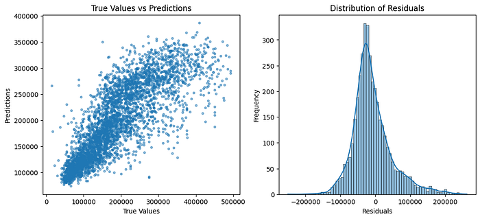
# R-squared (R2) Score: 0.64

The model does not perform extraordinarily well. We obtained a Mean-Absolute-Error of 43颏 US Dollars, which is quite high. The residuals are roughly normally distributed but seem to display a higher variance as the value of a house is higher.

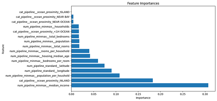
In terms of feature importance, the median house value, the category "INLAND" from our categorical variable ocean proximity as well as the population per household seem to be the most important features.

Conclusion

The model does not perform very well. Several improvement steps could be implemented. First of all, we could try another model such as XGBoost. Features like population could be log-transformed since they display a skewed distribution. But for now, we have a stable pipeline that we can also use for other projects.