This is the second group (Lenny and Rohan) entry in our journey to extend our knowledge of artificial intelligence and convey that knowledge in a simple, fun, and accessible manner. Learn more about our motives in this introduction post.

We are back! College applications and senior year have drained quite a bit of our free time, but we're still alive (albeit slightly sleep deprived).

Let's talk about a topic that we've been meaning to write about for a while but haven't gotten around to doing: convolutional neural networks.

Before we get started, you should try to familiarize yourself with "vanilla" neural networks. If you need a refresher, check out our neural networks and backpropogation mega-post from earlier this year. This is so you know the basics of machine learning, linear algebra, neural network architecture, cost functions, optimization methods, training/test sets, activation functions/what they do, softmax, etc.

Problem

Computer Vision

What is computer vision?

You probably guessed it: it's computers seeing things! Duh.

But "seeing" is a pretty vague term. Computer vision — which is really an interdisciplinary field — is about computers being able to gain high-level understandings and make conclusions, predictions, and/or statements from some kind of visual input.

Let's start talking about sub-problems in computer vision. Because, in reality, when we say "computer vision" we are not referring to one concrete task. Instead, we are referring to a group of tasks that machine learning has attempted (both successfully and less so) to solve. However, the most common task we hear about, and the one we will specifically look at in this article, is that of object classification. It's pretty much exactly what it sounds like: identifying and classifying the objects in an image.

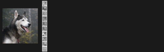
Let's demonstrate this with a cute picture.

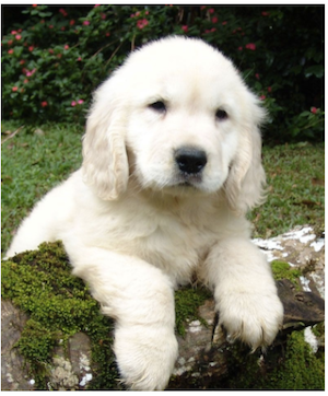
A successful object classification algorithm would look at this image and output that there is a "Dog" present in it. An even better classification algorithm may suggest "Puppy" as a more accurate or precise class of the object. "Flowers" and "Grass" may also be reasonable classifications if we're trying to look for all of the objects in an image.

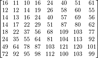
This is one of the hallmark problems in computer vision — being able to take an image or video and identify/classify the objects inside it. And it's not easy. Because, this is what the computer sees when it looks at that dog:

So… why do you care? And why should you care? Object classification, other than being a major step forward for understanding computer vision as a whole and furthering machine learning, has dozens of applications. Some of these applications are integral to your daily life, some are integral to the operation/growth of many companies, and some make the government or military run. Here's a small list of specific capabilities:

• Autonomous cars (they need to perceive the world around them)
• Facial detection/recognition
• Organizing photos (eg. Google and now Apple's photo app)

The same algorithm that can be used for object classification, however, can also be used to — for example — analyze an fMRI brain scan and make a predictive diagnosis on it. In this sense, the algorithm is not classifying an object but trying to look for patterns in the image that would make it similar to other fMRI scans it has seen before.

Computer vision has countless other sub-problems. Object segmentation is about figuring out where exactly different objects lie in an image. Scene parsing lets us look at an image as a whole to segment it into generic categories (sky, grass, road, etc.). When dealing with video, motion tracking helps figure out how a particular object moves from frame to frame.

Put simply, computer vision is a pretty big field. This article will mostly focus on classification, but CNNs are applicable to countless other problems as well.

Problem with Vanilla Neural Networks

Okay, cool. So we need an algorithm to do some computer vision — why not use a good ol' neural network? Surely, deep artificial neural networks, the almighty machine learning algorithm, would be able to succeed in computer vision!

Well, as it turns out, traditional neural networks don't work that well for computer vision. Actually, they really suck. Let's see why.

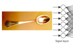
Imagine a neural network that takes an image as input and outputs a probability distribution over potential classes for the "primary" object it sees in the image. Let's pretend that each of the images we are feeding into this ANN is a closeup of said object against some background, like this:

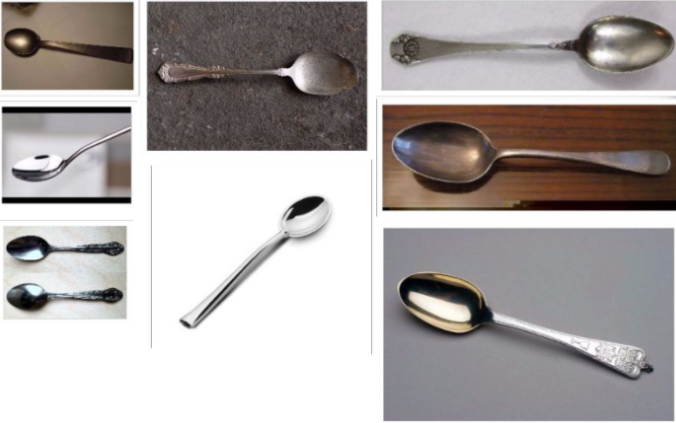
Let's now say we are trying to classify cutlery only (I think you Americans call it "silverware" or something). Our discrete classes will be represented by the probability in the individual output nodes of the ANN. Like this:

We'd expect a properly trained ANN's value in the "Spoon" output node to be the greatest, with "Spork" probably coming in second place.

Ok, so this all looks great. What's the issue? Well, here it is:

Turning an image into a bunch of separate input neurons isn't actually the problem. That's pretty easy to do — we could just treat each neuron as each separate pixel in the image. For simplicity's sake, let's convert the picture to grayscale, such that each pixel is represented by exactly one number between 0 (black) and 1 (white). We can then "flatten" this 2D array of pixel values into a 1D array (that is, just concatenate each sub-array to the previous one to make a long list of all the pixels), which corresponds to the input to our neural network.

Here's what that flattening process could look like visually:

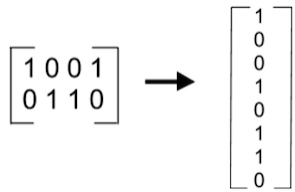
Let's just call this a pixel input vector. Now, let's consider — on a high level — what the ANN is doing.

First, we'll give it a lot of spoons. So. Many. Spoons. The network will try to look at all these spoons and try to figure out what makes a spoon a spoon based on patterns in the images (e.g. the reflection from the spoon head, the convex indent that is on the spoon head, the handle, etc.) We might also add images of forks and knives to understand concretely what makes a piece of cutlery NOT a spoon.

But, notice something. While inputting these images of different spoons, we would expect them to have similar pixel input vectors because they are all spoons. When a new image of a spoon comes along the ANN should be able to (abstractly and mathematically) say — "Hey, this looks similar to all the other spoon pixel input vectors I've seen…so it's probably a spoon!". It should be able to find distinct patterns in these pixel input vectors that it can use to ascertain what makes a certain pixel input vector likely to be that of a spoon. That's how any supervised machine learning algorithm or ANN should work.

However, this just isn't the case. The reality is, the pixel vectors of the following two images — even at grayscale — are completely different:

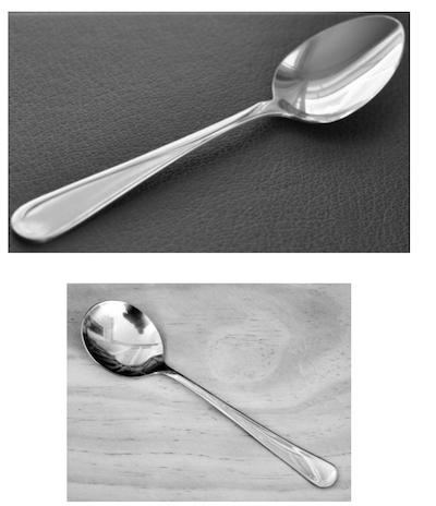
Yes, these are both images of a spoon, but they are different type of spoons, the indented parts have different reflections, the orientations are different, the angles are different, the backdrops are different — I could go on and on. As a result, the actual pixel input vector will not be even remotely similar. Thus, an ANN will have a hard time associating these two images.

And this is a really really simple example. In reality our images will be larger, noisier, and the objects may be at different places in the image and of different sizes. Put simply, ANNs just won't do very well at these tasks.

The reality is that it's not the individual pixels that tell us whether an image of a spoon is an image of a spoon — it's something much more abstract than that. It's the handle and the circular indent that we identify, for example. These are the "characteristics" of a spoon. And, ultimately, it's edges, lines, and corners that superimpose on each other to build out these characteristics. Operations on individual pixels aren't enough to let us figure out if these pixels represent a spoon. Instead, we need to figure out the pixel groupings that make these edges/lines/corners and see how groupings of those edges/lines/corners then go on to form the characteristics. Furthermore, flattening images into single vectors — though retaining information of the pixels — loses information such as the structure of the image. Our neural network would not be able to exploit this structure, which is certainly important information when it comes to recognizing objects.

However, this is not the only issue. It's also very valid to suggest that ANNs simply don't scale well to large images. If each value in the pixel input vector is fed into a separate node, we essentially are going to have a new input feature per pixel. Imagine a 200 x 200 grayscale image — that's 40,000 input features! That would mean something at least on the order of hundreds of thousands of weights per layer (if not more), which is simply infeasible. Such a large number of parameters would mean slow training and very likely overfitting as well.

Why pixels anyways, though?

Why input pixel values to the ANN? Why not choose and extract/compute our own features for classifying spoons?

Well, it could work (and that's exactly what we used to do), but human-constructed features are rarely as good as "learned" features. Sometimes we also just don't know how to come up with good features for certain objects. On top of that, if we want to truly solve computer vision, human-constructed features simply aren't a good approach — we want to build algorithms that can see and classify anything based on prior experience/training with that thing and without human intervention.

Really, this is the sort of thing that we want artificial intelligence to solve. And convolutional neural networks do it beautifully.

Moravec's Paradox

Before we go any further, you might be wondering: why is it so frikin' hard to get computers to see? We humans don't need to put any effort into it! When I see a computer in front of me, there is no hardcore processing or rationalization that my brain needs to undergo. I'm just like: "Yo, whose Macbook is that?"

Yet, why is it so hard for us to multiply 359 and 214.24 in our heads? (Try it, I dare you.) The dumbest, slowest computers can do it so easily, yet I'm 100% sure the common man would give up before even starting.

This highlights moravec's paradox: the discovery by researchers in artificial intelligence/robotics that high-level reasoning requires little computation for computers but great computation for humans, whilst low-level sensorimotor (fancy word — basically sense perception like seeing) skills are the opposite. Hans Moravec puts it straightforwardly:

It is comparatively easy to make computers exhibit adult level performance on intelligence tests or playing checkers, and difficult or impossible to give them the skills of a one-year-old when it comes to perception and mobility.

Marvin Minsky (R.I.P.) said it best, though:

In general, we're least aware of what our minds do best… we're more aware of simple processes that don't work well than of complex ones that work flawlessly.

This is an interesting observation because it's obviously so relevant to computer vision. An explanation offered by Moravec, though, is that we can attribute this all to evolution. Over the course of millions of years of human evolution by natural selection, our brains have increased in complexity and improved in design. Seamless object recognition and abstract thinking are potential examples of these.

Really, the oldest human skills like abstract thought, object identification through vision, and complex linguistic expression are largely unconscious processes (we don't really need to think to do them) and thus to us they seem very effortless to us. Over many many years, they have continued to evolve to make them so seamless. We should expect that these skills — being so old and so evolved/iterated upon — will take a lot of time to replicate in machines/computers. That is why this seeming "paradox" might not be a paradox at all.

Vision in the Brain

Unsurprisingly, these convolutional neural networks (and yes, we still haven't explained what those are — we're getting there, I promise) are heavily inspired by our own brains. So, it might behoove us to figure out how we humans look at stuff, and then derive a neural network architecture to mimic that. If you don't really care about any of this and just want to get to the good stuff, you should be OK to just skip this section and move on.

Still here? Good. Our visual system, like the rest of our nervous system, is composed largely of neurons. Biological neurons do pretty much the same thing as artificial neurons in our ANNs; they take inputs from other neurons, and can choose to emit an output based on these inputs. Unlike ANNs, the inputs and outputs are a binary on/off signal instead of a real number, but neurons can vary the firing rate (the rate at which they send an output signal). When we say a neuron is "excited," that just means its firing signals like there's no tomorrow.

Ok, now let's talk about how we go from light to neurons. Humans see things through their eyes: photons shoot towards your cornea, through your pupil, and hit the retina at the back of your eyeball. Photoreceptor cells (rods, cones) in your retina get excited when they see light and color, and that eventually works its way to your retinal ganglion cells.

It's in these retinal ganglion cells where things first start to get interesting. Each retinal ganglion cell takes inputs from a cluster of photoreceptors, representing a small region of your vision. Your retinal ganglion cells divide this region into a "central zone" and a "peripheral zone" around the center; if the cell gets the right amount of light in each of these regions, it will start firing to let the downstream parts of your vision pathway know it sees something. Concretely, there are two types of cells: on-center and off-center. When on-center cells see light in the middle of their respective region, they get all excited and start firing. When off-center cells see light around the center, they too get excited. The takeaway here is that each cell responds to a certain pattern in its input, which we can build off later on to detect more complicated patterns. We'll see how that works in a minute.

An important thing to note here is that every cell is only affected by a small region of your vision. The firing rate might be heavily influenced by the amount of light hitting that small part of your retina, but outside of that region the firing rate of that cell is unaffected. The region of your vision that influences a particular cell is called a receptive field (RF). There was a famous experiment by Hubel & Wiesel that demonstrated this concept: by recording the signals coming out of one of these cells (converted to audible beeps in the following video), they showed that one of these cells is only responsive to a particular region of your vision.

(Now comes the part where I think I can design my own diagrams.) Imagine all of your retinal ganglion cells organized into a grid based on the region of your vision that they represent, like so:

Let's pretend we see something: a bright light directed at the center of our vision. The cells in the center of our field of view get all excited, but the rest still have no idea anything's changed — receptive fields at work!

If we take a step back and look at this a bit more abstractly, what we're really doing is transforming the data we're getting. Initially, our "data" was the light coming into our eye; while this representation was rich with detail, it was hard to get to the "core" of what we were really seeing. Using the photoreceptors and retinal ganglion cells, we can reduce this representation to something more meaningful: "where is there light?" Other cells early on in the vision pathway can pick up unique colors and basic patterns that help round out this new representation with more information that we can use to eventually pick out individual objects and shapes.

The signals from your retinal ganglion cells eventually make their way through something called the LGN and into your primary visual cortex (affectionately called "V1"). Like the cells in your retina, V1 cells look at just small region of their input. Building off of the work done in your retina to pick out light and color in what we're seeing, these V1 cells can start looking for things like lines and patterns; essentially building a "representation" of the data that's a little more abstract and higher-level. Once again, Hubel & Wiesel come to the rescue with a demonstration:

Ho-ho-ho, I think we have ourselves another transformation! Our new grid of cell activations will light up when it sees a line or border, and stay quiet otherwise. I think you can see where we are going from here — once we have "maps" of different patterns and lines in the image, it becomes easier to look for shapes and borders. From there, we can begin to identify primitive objects and more complex shapes. Finally, we can look for and identify complete objects in our vision. Each transformation builds on the previous representation; it's hard to identify that we are looking at a cat from raw photoreceptor inputs, but if we are looking at borders, shapes, and textures it suddenly becomes quite clear what we're looking at.

It's this hierarchical structure of our visual system that enables us to see and identify so many different objects. As you're about to see, the same concept transfers beautifully to neural networks.

Architecture of a Convolutional Neural Network

So the problem with using a normal neural network is that it's basically impossible to extract any meaningful features from a bunch of pixels directly. To solve this, a CNN uses a hierarchical approach to learn feature detectors that are increasingly abstract. For example, a CNN might start by looking for lines and borders in our image. From there, it can look for basic shapes and curves. Oh hey, those curves kind of look like an ear and a nose. A face tends to have ears and a nose. Hey, maybe we're looking at a person!

Let's put this all into more concrete terms. If you read the last section, you'll recall that the cells in our retina have a receptive field within your field of view — each cell only responds to activity in a small portion of your vision. Furthermore, recall that each cell only activates for a specific pattern within that region. In a convolutional neural network, we have a very similar principle — a convolutional kernel (or filter) describes an individual pattern, which is then applied to every part of our image.

With CNNs, we talk about volumes instead of normal vectors. Instead of a 1-D vector of numbers that we pass into our network, it's conceptually easier to envision our image as a 100 x 100 x 3 volume of numbers (100 pixels wide, 100 pixels tall, and 3 channels [R, G, B] deep for the colors).

We make these transformations using convolutional layers. In a normal fully-connected layer, we would have one weight per input for each neuron; in a convolutional layer, we instead learn the weights of a filter that we apply to every part of our input volume. If our initial input volume is 100 x 100 x 3, we might learn a 5 x 5 x 3 filter that we apply to each individual part/sub-section of our image.

What do we mean by "apply"? Quite simply, we take the dot-product of our filter with the region of our image. We start with the top-left corner, and apply our 5 x 5 x 3 filter to get a single number (intuitively, this number represents how strongly that region "matches" our filter). We then shift over our filter by 1, and take another dot-product. This gives us another value, which we pass through our non-linear activation function. We combine all of these dot-products into a brand new volume (which we call a "feature map").

Make sense so far? If not, here's a GIF of a 3 x 3 filter in action (wait for it to begin animating):

A few extra things to note: I just said that we shift over our filter by 1 every time we take a dot-product, but we can actually shift it over by as little or as much as we want; the number of spots we move over is called the stride. We should also discuss the size of our new volume we get; intuitively, the size of the new volume will be smaller than the input (see the animation above if you need convincing). If we don't want the volume to get smaller with every subsequent convolutional layer, we can add a layer of padding around the input before we apply our convolutions. For example, if we use a padding of two, we will add a two-pixel-wide border of zeros around our input, and then do our convolution generate our feature map. We can use this handy equation for computing the size of our new output:

Let's reiterate: we have our input image, which we'll say is 100 pixels long by 100 pixels wide. Each pixel has three numbers associated with it: a red channel, a green channel, and a blue channel. We represent our image as a three-dimensional volume of numbers (100 x 100 x 3). We learn a filter (we'll explain how to learn the filter in a bit), which we apply to every part of our image, giving us a new volume (assuming we used the appropriate padding, we'll assume this new feature map has the shape 100 x 100 x 1). This process of applying the same filter all over the image is known as a "convolution" (hence the term, "convolutional neural network").

Why does this work? Let's say the filter we learned was great at detecting edges in our image. This means that our new "feature map" would light up wherever we have a border, essentially giving us an outline of what we're looking at. This kind of representation is far more useful to our network than the color of each pixel; it lets us extract more meaningful features from our image further down the line.

That's basically the gist of it. The last remaining detail is that each convolutional layer can actually have multiple filters in it; instead of convolving just one filter and creating just one filter map, we learn many filters (often as many as hundreds per layer) and apply each one to the input volume. This gives us as many feature maps as we have many filters, which we can stick together to create a larger volume. So if our initial input is 100 x 100 x 3, and our first convolutional layer has 192 filters, our output volume will have size 100 x 100 x 192 (again, assuming that the stride and padding are configured appropriately to prevent the output size from shrinking). Each filter map will give us a different unique perspective on the image (unique patterns, lines, borders, etc.), which when combined together give us a new representation of the image which is far more meaningful than the initial image or any individual feature map.

The next convolutional layer will take this 100 x 100 x 192 input and apply its own set of filters to the image of size n x n x 192 (notice that, while the size of the filter can be whatever we want, it extends through every feature map from our input volume). Each successive convolutional layer can build off of the work of the previous one; using the borders we found in the first layer, we can find unique shapes and curves in the second layer. The third layer can find even more abstract and meaningful features. But eventually, we need to start reducing the size of our representation as the features we learn span a larger and larger region of our image. This is where pooling layers come in.

Pooling layers are a way to reduce the size of our volume as it flows through our network. We'll start by looking at one particular kind of pooling layer, the max-pooling layer, but the same principle applies to related layers, like average-pooling.

Quite simply, our max-pooling layer takes a small subsection (say, 2 x 2) of each filter map in its input volume, and only takes the largest value from that subsection. Perhaps this is best explained with a picture:

Let's go back to our 100 x 100 x 192 output of our first convolutional layer and apply a 2 x 2 max pooling. Our new output will have size 50 x 50 x 192 (notice that it keeps the number of feature maps the same, but reduces the two other dimensions by a factor of 2). Our pooling layer has two hyperparameters: the size (2 in the previous example) and the stride (also 2 in the previous example). We can compute the size of our output using the following formula:

And that's it. Notice that pooling layers have no parameters (only hyperparameters) — they simply apply a function to regions of its input. Intuitively, you can think about pooling layers as reducing the "resolution" of our input volume; if we go back to our feature map of lines, and apply a pooling operation, we will end up with basically the same picture just with fewer "pixels". This is called down sampling.

Generally speaking, the stride and size of a pooling layer are the same, but there's nothing stopping you from creating an "overlapping" pooling layer (as we'll see in the case study that follows) where the size is greater than the stride.

Convolutional and pooling layers make up the bulk of most CNNs, but we still need to somehow come up with a probability distribution over classes. We can do this with our normal fully-connected layers we are so used to seeing in regular neural networks. Our last convolutional or pooling layer gives us one last output volume, with very high-level and abstract features (ears, eyes, leaves, etc.). If we connect a fully-connected layer to each value in our volume, we can train one neuron per class (with a softmax stuck on the end to convert it into a probability distribution). If we want an extra little bit of representational power, we can stick on some extra fully-connected layers before our final output layer.

So now, how do we actually learn or define these filters and their specifically weights/biases? Our objective is to find filters that minimize error/cost and in doing so maximize the percentage of correctly classified images. We of course use the backpropagation algorithm to compute our derivatives and then apply a first-order or second-order optimization algorithm like stochastic gradient descent or L-BFGS respectively. The cost function we use can be any typical one, for example cross-entropy (or "logistic") loss.

I'll wrap this up with a little note on transfer learning (which applies to neural networks in general, but is especially common when training CNN models). You need a lot of data to train one of these networks successfully, and depending on the problem you're solving, there isn't always all that much data to go around. Data augmentation can help, but nothing beats a ginormous dataset with hours of GPU training time. But because of the nature of pictures, a lot of the features that CNNs are learn are fairly generic; the lines, patterns, textures, and so on that a network learns to look for can often be found in most images, even in categories it may not have been explicitly trained on. For this reason, it's common to start training with a popular architecture and an already-trained model; if you freeze the weights of the convolutional layers and just train some fully-connected layers on top of them, you can learn to recognize an entirely different distribution of objects with far fewer images.

And that's it! Not so bad, right?

Why this works (briefly)

Let's take a quick look at why ConvNets work and what they really do. We briefly mentioned before that they can learn weights for feature detectors that are increasingly abstract; perhaps they first start by detecting the edges, lines, and corners in parts of an image via the initial convolution layers and then proceed to, in the later convolution layers, recognize things like noses, eyes, bike handles (just a random thought) that can then be used to figure out exactly what the object is.

The fully connected layer(s) at the very end let us combine these individual features and figure out what exactly we're looking at. Another approach, as mentioned before, would have been to use a normal neural network with hand-crafted featured as inputs, instead of the convolutional layers. Obviously, finding and computing said features is extremely difficult, very time consuming, or simply not possible. CNNs fix this by finding effective feature detectors themselves. The point of using CNNs is that by training these convolution layers they can create their own feature detectors (ie. learning that seeing a bike handle might be a good way of figuring out that we're looking at a bike) that can then be applied to a fully connected ANN-like layer at the end.

A really cool way to demonstrate this is to extract the feature maps from each of the hidden layers and treat them as pixels that we can visually interpret. You can't see the actual contents of the following GIF up close but this is a good visualization of said feature maps from the original image and how they lead us to the end classification:

If we look at how the feature maps change as we go deeper and deeper into the network, we see that they quickly shift from easily interpretable (picking out basic textures and borders) to much less so (where each feature map might look for the presence of eyes or ears, for example).

However, if we look at the actual features that each feature map is looking for, we find that as we go further into our network they quickly transition from low-level borders and shapes to higher-level features and unique facial characteristics.

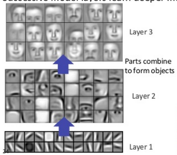
Ultimately, this is the point of the filter. Instead of looking at the image as a whole, we can look for low-level features — edges, corners, lines, borders — in a small region of the input. From these low-level features, we can "build up" and look for slightly more complex features in a slightly larger region of the image. That's why ConvNets work—the spatial convolution let us pick out small features and then work our way up to bigger ones. Once we have these greater abstractions it becomes pretty easy to classify.

CNNs are undoubtedly sort of automagical and black box (like a lot of deep learning) but they work really well. I highly encourage (in fact—I mandate!) that you watch the following YouTube video. It should make this explanation very intuitive.

Alright—now, let's take a look at some of the datasets and CNNs that are used in practice!

Case Study

ImageNet

OK, so now we're gonna take a look at an example. That is, how have some of the most successful CNNs been architected? How does one even get the data for training CNNs, and what are the kind of results that modern day networks achieve?

To answer these questions, we'll take a look at ImageNet. What is ImageNet? According to the website:

"ImageNet is an image database organized according to the WordNet hierarchy (currently only the nouns), in which each node of the hierarchy is depicted by hundreds and thousands of images. Currently we have an average of over five hundred images per node. We hope ImageNet will become a useful resource for researchers, educators, students and all of you who share our passion for pictures."

Basically, ImageNet is an open source (free) database of images with words/captions associated to them. Obviously, if you want to perform image classification (where you take an image and spit out the caption[s]/words associated to the main object[s] in the image), this seems like the perfect resource. In fact, as of 2016 (ImageNet began in 2010), there are over 15 million high-resolution, labeled images — meaning paired with crowd-sourced hand-annotated (yes, hand-annotated!) captions — from 22,000 different categories. Now that's a lot of training data for any sort of CNN out there!

ImageNet was started by students/faculty at Stanford University and the Stanford Vision Lab to collect data for computer vision algorithms — CNNs obviously included. The project continues to grow in an effort to help grow the field of computer vision and increase

Since inception, ImageNet has hosted an annual competition called the ImageNet Large Scale Visual Recognition Challenge (ILSVCR for short but I'm not sure who could memorize that acronym). In said competition, research teams (from institutions and companies) submit programs that perform object classification and detection on scenes/images from the ImageNet database. In 2010, a good classification error hovered around 25%. In 2012, the first year that a convolutional neural network won the competition, that almost halved to 16% (CNNs have dominated the leaderboard ever since). Now, the error rates are in the single digits, and researchers have reported that these error rates are in fact lower than human error rates! Of course, in context this means little since humans are still the best at contextual reasoning, not to mention the fact that we can recognize a lot more classes than ImageNet has. But it's still impressive.

In ILSVCR, models are trained on 1.2 million images in 1000 categories (hence the "Large Scale" part of the name). The task is to make 5 guesses, sorted by confidence/probability, about the potential label of input images:

You may see two separate measures of error: "top-1 error" and "top-5 error". Top-1 error occurs if the actual object in an image is not the most probable outcome class that the CNN produces. Top-5 error occurs if the actual object in an image is not in the five most probable outcome classes that the CNN produces.

Fun fact: in 2015 Baidu was caught cheating in the competition.

AlexNet

AlexNet was a deep CNN model created by Alex Krizhevsky (a student at UToronto) that, as mentioned earlier, took the error percent rate from the mid 20s to the mid 10s (which is a huge deal) in 2012's ILSVCR. AlexNet, however, isn't just any vanilla CNN you can throw together in 2 hours of hacking — there are many features that distinguish it from a typical convolutional neural network and I'll talk about them in this section.

Some high-level overview about AlexNet's architecture:

• It has 7 hidden layers (9 layers with input and output)
• 650,000 neurons in total
• 60 million parameters in total
• 630 million connections in total

Some more info:

• ReLUs are used as the activation function (Rectified Linear Units) — make sure you know what this is*
• It uses overlapping pooling layers
• Dropout is used to promote weight sharing and prevent overfitting
• Randomly extracted 224 x 224 patches for more data

*Ok but if you really forgot what they are (and haven't checked out our "Vanishing gradient problem" article) then it's a non-saturating (that is, the gradients don't die off) and non-linear activation function. The equation is ReLU(x) = max(0, x). If nothing you just read makes sense, I guess that's a prompt to go read the other article! ReLU is helpful; a 4 layer CNN with ReLUs can converge up to six times faster than an equivalent network with logistic/tanh neurons on the CIFAR-10 dataset. ReLU layers exist independently of convolutional layers.

A visual representation of the entire architecture follows:

There are 5 convolutional layers after the input, followed by 3 fully-connected layers (that is, just a regular ANN), and finally a 1000-way softmax for the output (to give us a probability for each of the 1000 classes in the 2012 challenge). If we fed in the leopard image above, we'd hope that the CNN would have the "Leopard" class with the highest output probability.

Now, let's look at each individual layer in the CNN and their features/role:

This is the first convolutional and hidden layer. In this layer, the convolutional filter convolves around the input image volume of size 227 x 227 x 3 with 96 11 x 11 x 3 filters with a stride of 4 and no padding. Using the equation we brought up earlier, we can figure out the size of our output volume: (227–11)/4 + 1 = 55. Because we have 96 filters, the output of the layer is ultimately 55 x 55 x 96. So, the first layer of AlexNet convolves around a 277 x 227 x 3 input image and outputs a 55 x 55 x 96 tensor as input for the next convolutional layer. Here's a nice definition of a "tensor" from Google, by the way:

A mathematical object analogous to but more general than a vector, represented by an array of components that are functions of the coordinates of a space.

Training for AlexNet also occurred on multiple (well, two) GPUs, but not much explanation needed here. The arrows that point to inter-GPU connections show connections that are being trained across different GPUs and intra-GPU connections show the ones being trained on the same GPU.

Before we looked at pooling layers in CNNs. AlexNet does use pooling — in particular it uses max pooling with overlapping. According to Krizhevsky, overlapping pooling slightly reduces error rates and overfitting as well (by about 0.4%.)

Now let's take a look at an overview of the full architecture of AlexNet:

We start with the previously described convolutional layer. Next comes a normalization layer (known as a Local Response Normalization — this isn't used all that much anymore, so we won't go into much detail here). Next comes a 2 x 2 max pooling layer. This block is repeated. Following that, we have three convolutional layers of smaller filter size (now 3 x 3 instead of 11 x 11) and then another max pooling layer. Then, we have two fully connected ReLU layers. Lastly, we have a fully connected softmax layer that outputs 1000 values (which is the probability distribution over the 1000 classes) from the down sampled, convolved, and basically broken down representation of the image.

Whew, that was a pretty long case study. AlexNet is some good stuff. There are some small extra techniques employed, mostly related to preventing overfitting, but I won't go into it — it isn't necessary at this point. Dropout, data augmentation, and modifications to the softmax algorithm are the notable mentions here. Finally, stochastic gradient descent with momentum (don't worry if you don't know what this is, but I think it's explained in our ANN article) was used as the optimization algorithm.

OK, now for some fun stats:

• AlexNet took 5–6 days to train
• It was trained on two NVIDIA GTX 580 3GB GPUs
• A top-5 test error of 15.3% was achieved (obviously 2015's competition had better results since this was 2012, but this was a big deal back then)

OK, now for some more fun: example classification results! This is actually really cool.

The top shows the actual image, in the middle shows the object present in the image, and the bottom shows the top-5 most probable objects that the algorithm has classified. The pink/red bar shows shows the class in the prediction/classification that corresponds with the actual label.

And that's AlexNet!

Implementing a CNN in TensorFlow

If you're thinking: "Rohan, dude, dope, CNNs sound like THE BOMB, but how do I actually make them?"

First of all, I agree with you. CNNs are the bomb. As for making them, lemme show you. We'll be, in particular, using TensorFlow, a popular "Open Source Software Library for Machine Intelligence" created and maintained by Google.

The following code, in Python, demonstrates the implementation of CNNs with TensorFlow (obviously make sure to install TensorFlow first, instructions are on their site). The CNN we'll be making is specifically being applied to MNIST: a dataset of handwritten numbers and their corresponding label. Thus, instead of object classification we are classifying a number (as a result there are much fewer classes; just 0, 1, 2, 3, 4, 5, 6, 7, 8, and 9) based on an image of said letter/number. This is useful for OCR.

The code is taken from TensorFlow's official tutorial on Deep MNIST implementation. We're going to build a CNN with the following architecture:

1. Convolutional layer
2. ReLU layer
3. Pooling layer
4. Convolutional layer
5. ReLU layer
6. Pooling layer
7. ReLU fully connected layer
8. Softmax fully connected layer

We also use dropout for regularization.

The following code downloads the MNIST data:

from tensorflow.examples.tutorials.mnist import input_data
mnist = input_data.read_data_sets('MNIST_data', one_hot=True)

The next 2 lines of code sets up a TensorFlow session:

import tensorflow as tf
sess = tf.InteractiveSession()

The first line of code is easy to understand: we just import TensorFlow as "tf". Then we create a new "InteractiveSession". Sounds fancy, but what is it? Well, this concept is perhaps at the core of TensorFlow. It's the idea of representing computations as graphs. Nodes in said graphs are called ops (short for operations), and each op takes zero or more Tensors, performs some computation, and produces zero or more Tensors. These "Tensors" are typed multi-dimensional arrays—or simply put, mathematical tensors—the dimensionality of which we will look at soon.

A lot of that description was pulled from TensorFlow's site, however I'm gonna make it simpler for you here. After all, that's one of the goals of this blog.

In TensorFlow, mathematical operations that you perform on tensors aren't actually performed. Instead, they're added to a computational graph that defines what kinds of computations we are doing. So we first build our network by defining all of our operations (which are the convolutional neural network layers eg. convolutional/pooling/ReLU etc.), and that creates our graph. Then, when we're ready to use our network, we tell TensorFlow to run the graph that we've created, giving it actual values to plug in to the tensors and letting it compute the rest. It's pretty dope, in my opinion! But, if it doesn't quite make sense yet don't worry, you'll see what I mean as we keep going.

OK, so now we're going to define two functions to help us out:

def weight_variable(shape):
 initial = tf.truncated_normal(shape, stddev=0.1)
 return tf.Variable(initial)
def bias_variable(shape):
 initial = tf.constant(0.1, shape=shape)
 return tf.Variable(initial)

The first function initializes weights based on a given shape/dimension. Obviously, to set up a CNN we're gonna need a lot of weights/biases. Generally, we don't set these values to zero but instead add a small amount of noise to prevent symmetry and premature convergence/high error on neural networks: that's exactly what the truncated_normal function does, and we specify a standard deviation of 0.1 to the normal distribution.

We put our weights into a TensorFlow variable. Remember that TensorFlow doesn't deal with values directly; it deals with "operations" on a "computational graph". A Variable is just a special operation that doesn't take any inputs and returns the value that sits inside the variable. The variable won't actually have a value inside of it until we run the graph.

The second function creates a bias variable, again based on a given shape. We initialize it to a constant value of .1 (ReLU cuts off any activations <0, so giving it a slight positive bias prevents dead neurons).

We'll now write functions to create reusable layers—that is, the convolutional and max pooling layers. The code follows for the convolutional layer:

def conv2d(x, W):
 return tf.nn.conv2d(x, W, strides=[1, 1, 1, 1], padding='SAME')

This function, aptly titled "conv2d", creates a 2D convolutional layer. A 2D convolutional layer uses a 2D filter, which is a filter that convolves in the horizontal and vertical direction/dimension of an image. Note that we do not convolve in the depth/z-axis of an image (the channels).

The tf.nn.conv2d function takes as input a 4-D input tensor (which corresponds to variable x, which will be the input of the layer). Wait… but why 4-D? "I thought you said images were 3D volumes?", you're probably thinking. I hear you. Worry not. Basically, when we train a convolutional neural network, we want to train it on a batch of images. You don't just wanna train it on one image/corresponding label at a time, just like a (properly vectorized) linear regression algorithm wouldn't train on one data point at once. Thus, we collect a batch of 3D tensors and put it into a 4D tensor. Obviously, this means that all images must be of the same dimension. The dimension of the entire input tensor is now: NUMBER_OF_IMAGES x STANDARD_IMAGE_WIDTH x STANDARD_IMAGE_HEIGHT x STANDARD_IMAGE_CHANNEL. The 2d convolution layer still only operates/convolves on the height and width.

Ok, cool.

The W parameter corresponds to our convolving filter — these are of course, weights. They are TensorFlow Variables that can be generated using the function we wrote earlier on. Now, the strides argument (which we set explicitly to an array of four 1s) is sort of confusing: isn't there just… one stride? Maybe two? But why four? Ok, so here's what's up: since we have a four dimensional tensor input, we have a four dimensional stride input that corresponds to the stride value used for each axis. (Yes, you can technically have a different stride for each dimension, although I'm not quite sure why one would want that. But hey, I'm not here to judge.) Because this is a 2D convolution, TensorFlow actually requires that the first and last strides, corresponding to the batch dimension and the channel dimension, be set to 1.

Therefore, strides[1] and strides[2] can just be set to the stride values for the x and y axis. Why TensorFlow has you input an array of four values, only to literally force two of those values to be 1, confuses me as well. Don't worry.

We set the stride for the x and y axis to just be one. padding='SAME' is sort of confusing as well. Basically, this is the argument we pass to specify the zero padding for the convolutional layer. With TensorFlow, you can pass one of two arguments:

• SAME
• VALID

Again, this confuses the hell out of me. SAME is the most common one, apparently. A more thorough exploration into the differences between these not so aptly titled arguments are available on one of their documentation pages.

The code follows for the max pooling layer:

def max_pool_2x2(x):
 return tf.nn.max_pool(x, ksize=[1, 2, 2, 1],
 strides=[1, 2, 2, 1], padding='SAME')

No need to spend too much time on this. We pass the input x, and the ksize parameter (once again we set the first and fourth value to 1) is the size of each max pooling sub-region (2 x 2 here), whilst we use stride of value 2. We use the same padding as before.

At this point we've defined all the functions we need to, and we can construct our neural network in our computation graph. But before that, we need to write the code to create placeholders for our training set data values:

x = tf.placeholder(tf.float32, shape=[None, 784])
y_ = tf.placeholder(tf.float32, shape=[None, 10])

Remember, these are not specific values (therefore they are placeholders). We need a way to feed in our values when TensorFlow starts executing our computation graph; we do this with a placeholder. When we actually run the graph (and we'll see how in a bit), we can specify which values we want these placeholders to have.

The input x is a 2D tensor of floating point numbers, with the dimension [None, 784]. 784 is the number of pixels in a single flattened MNIST image. TensorFlow gives us these images as a 1D vector, but we will reshape them back into a square before we give them to our CNN. Another little thing to note is that MNIST images are in grayscale, so it's 2D rather than 3D because the channels dimension is just 1. None means that the first dimension can be of any size. In our case, that dimension corresponds to the batch size we use.

y_, the labels or known output of the training data, is a "one-hot vector" of 10 values. What does a one-hot vector mean? It's actually really simple; one-hot vectors — aptly titled by the way, which y'all know I really appreciate — are just vectors that contain the value of 1 in any given single position and the value of 0 in every other position. There are 10 values because there are 10 possible output classes of the CNN with MNIST: 0, 1, 2, 3, 4, 5, 6, 7, 8, and 9. When it comes to the output of the network, there will a probability/confidence distribution over each of these classes. However, the output of the input training set data is… certain, so one of the values will be 1 and the rest will be zero.

Let's get on to creating our first convolutional layer! We'll first create the weights and biases (the convolutional filter) for this layer.

W_conv1 = weight_variable([5, 5, 1, 32])
b_conv1 = bias_variable([32])

We use the functions we've already defined to create these weights/the bias. The weight tensor has a shape of [5, 5, 1, 32] because our filter is of size 5 x 5 (pretty standard). We only have one channel for grayscale and it's a 2D convolution. The final value, 32, is the number of output channels that we have — the number of features or "feature maps" that will be produced from this convolution. Basically, a 5 x 5 x 32 tensor will be outputted from this convolutional layer that will be inputted to the next one. We also create our bias variable with a component for each output channel.

Next, we take our tensor of n x 784 flattened image vectors and reshape them back to their original 28 x 28 dimensions:

x_image = tf.reshape(x, [-1,28,28,1])

This is again important because CNNs can exploit and learn from the structure of images. The -1 here just means it does not change, because we retain the batch size.

We now convolve x_image in 2D with our weights and add our biases using the function we created earlier:

h_conv1 = conv2d(x_image, W_conv1) + b_conv1

Following this, we apply the ReLU activation function and then do a 2 x 2 max pooling operation:

h_conv1 = tf.nn.relu(h_conv1)
h_pool1 = max_pool_2x2(h_conv1)

That's the first layer (or first three, if you think of ReLU/pooling as separate) done! Let's take a quick look at the size of our current image. Before, it was 28 x 28. However, with our convolution and pooling, it should be down sampled. We apply the following equation that was explored before:

Where W is the dimension of the original image, F is the filter size, P is the padding size, and S is the stride value. We sub in:

• W = 28
• F = 5
• P = 2
• S = 1

To get a value of 28. That's right — the image size doesn't change. However, we're forgetting that we also need to apply the pooling equation:

Where W is the original image size, F is the pooling filter size, and S is the stride value. We sub in, as per the code in our functions:

• W = 28
• F = 2
• S = 2

Now we get to an image dimension of 14. So, after the first convolution/pooling layer, our image has been down sampled to 14 x 14.

Next we have a second convolutional layer that, instead of 32, now creates 64 features for each 5 x 5 filter and then applies ReLU/max pooling.

W_conv2 = weight_variable([5, 5, 32, 64])
b_conv2 = bias_variable([64])
h_conv2 = tf.nn.relu(conv2d(h_pool1, W_conv2) + b_conv2)
h_pool2 = max_pool_2x2(h_conv2)

Our image is now down sampled to 7 x 7 (if you repeat the same calculations as before). Since we have 64 output channels, we now have 7*7*64 = 3136 values. Next, we have a fully connected layer with 1024 neurons. That is, 3136 output values are flattened and then directly connected to 1024 neurons. The number 1024 is arbitrary and has been chosen based on positive empirical results.

We first create the weights/biases:

W_fc1 = weight_variable([7 * 7 * 64, 1024])
b_fc1 = bias_variable([1024])

Then we take the output of our previous layer (the pooling layer) and reshape (flatten here) it into a batch of vectors of 3136 values.

h_pool2_flat = tf.reshape(h_pool2, [-1, 7*7*64])

Following this, we perform the fully-connected layer operation of multiplying our values by the weight matrix ("matmul" stands for matrix multiplication) and then adding the biases. This is like Machine Learning 101 😛

h_fc1 = tf.matmul(h_pool2_flat, W_fc1) + b_fc1

Finally, we apply ReLU:

h_fc1 = tf.nn.relu(h_fc1)

To reduce overfitting, we apply this technique called "dropout". No worries if you don't know what it is, very little code is required to implement it. On a high level, dropout randomly turns off some of the neurons while training to increase the independence of each of them individually and reduce dependence on each other and temper the influence of a given neuron. In general, this enables a neural network to generalize better because several independent representations of patterns can be learned. The variable keep_prob in the following code is an aptly-titled value that states the probability of any given neuron being kept/left on and not turned off. We'll explicitly set that value when we run the interactive session.

keep_prob = tf.placeholder(tf.float32)
h_fc1_drop = tf.nn.dropout(h_fc1, keep_prob)

We're almost done! Finally, we'll add a fully-connected softmax layer that can turn the output from 1024 neurons into a probability distribution over the 10 classes of number characters.

We create the weights as per usual:

W_fc2 = weight_variable([1024, 10])
b_fc2 = bias_variable([10])

Now we create y_conv, our final output that performs a fully-connected operation on the dropout and following that a softmax.

y_conv = tf.nn.softmax(tf.matmul(h_fc1_drop, W_fc2) + b_fc2)

Cool! You've just constructed your very first convolutional neural network. You're not just a builder — you're an architect!

But we're not done yet. Now let's go ahead and train/evaluate our model, and learn how well it performs.

cross_entropy = tf.reduce_mean(-tf.reduce_sum(y_ * tf.log(y_conv), reduction_indices=[1]))

The line of code above is essentially our cost function, where we aim to make y_ (our known output) and y_conv (out estimated/predicted output) as similar as possible.

train_step = tf.train.AdamOptimizer(1e-4).minimize(cross_entropy)

This line of code defines an iteration of optimization (using the first-order optimization method called Adam) with a step size of 0.0001 by minimizing the output of the cost function we just defined.

correct_prediction = tf.equal(tf.argmax(y_conv,1), tf.argmax(y_,1))

This is a vector of booleans where 1 indicates a correct prediction (that is, for that image in the batch y_conv and y_ both chose the same class as the output number character class.) y_conv is continuous rather than discrete like y_, but the function argmax returns the index with the highest value (exactly 1 for y_ and closest to 1 for y_conv) so that's not an issue here. We don't check if the values are exactly equal.

accuracy = tf.reduce_mean(tf.cast(correct_prediction, tf.float32))

This line of code just gets our overall accuracy by calculating the mean of our predictions.

OK. You ready for this? Let's finally run our session!

sess.run(tf.initialize_all_variables())

Now let's input our data:

for i in xrange(20000):
 batch = mnist.train.next_batch(50)
if i % 100 == 0:
 train_accuracy = accuracy.eval(feed_dict={
 x:batch[0], y_: batch[1], keep_prob: 1.0})
 print("step %d, training accuracy %g"%(i, train_accuracy))
train_step.run(feed_dict={x: batch[0], y_: batch[1], keep_prob: 0.5})

20,000 iterations in the for loop is basically the batch size (which we have set to 50) multiplied by the number of steps of the training/optimization method (which we have set to 400). You can change these numbers as you wish.

In each iteration, we get our next batch (remember we are training in batches) and then proceed with our training/optimization step using train_step. We pass to train_step the argument feed_dict, which contains the 50 x input images, 50 y_ known output classes, and the keep_prob for dropout which is 0.50.

Also, every 100 overall iterations (that's the i % 100 == 0 if-statement), we log the current training accuracy for the batch (which would be every 2 training/optimization steps for each individual batch since 100 / 2 = 50) and then print that out. This helps us keep track of how the accuracy is changing over time, but we don't want to spam by calculating and outputting the accuracy every iteration because it's unnecessary and would slow things down a lot.

Finally, once we have finished optimizing on our training set, we go ahead and log our test set accuracy:

print("test accuracy %g" % accuracy.eval(feed_dict={
 x: mnist.test.images, y_: mnist.test.labels, keep_prob: 1.0}))

You should get up to 99.2% accuracy if you leave it running for a while (and if you're okay with your fans goin' crazy!). Hope you had fun with that. The theory and math behind CNNs and machine learning in general is great, but implementing and getting your OWN machine to learn is even cooler 😎

Also, for this small CNN, performance is nearly identical regardless of whether dropout is used. Dropout is really good at reducing overfitting, but it's more relevant and effective with very large industrial-setting networks.

TIP: if you get an error about some UTF-8 locale stuff, enter this into your command line/Terminal (not Python):

export LC_ALL=C

Here's all the code pieced together.

Conclusion

Yea, so that was probably a long read! Hope you learned something about convolutional neural networks and that they're not magic but instead just a really cool and ingenious advancement in computer vision.

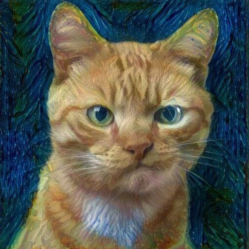
To conclude, here's an image of a cute cat that has been painted over in a really dream-like/psychedelic fashion by a CNN. It's done by Google's DeepDream program. Maybe this is something we can talk about in the future?

Til' next time, when we dive head first into the recurrent neural network! 🍺