Hey everyone ! I'm Pankaj Chouhan, and I've been on a machine learning journey lately. One algorithm that really caught my attention is the

Decision Tree

it's simple, intuitive, and feels like how we humans make decisions every day. Imagine you're deciding whether to play football outside :

Is it raining ?

Too windy ?

Enough friends available ?

You ask step-by-step questions to decide. That's exactly how Decision Trees work in machine learning! They're powerful tools for breaking problems into smaller, manageable questions to predict outcomes.

In this guide, I'll walk you through what Decision Trees are, how they work, and the key ideas behind them — like entropy, Gini Index, and pruning. I'll also share Python examples using the Iris dataset and a custom student example to make it crystal clear. Whether you're a student or just curious about ML, this is for you. Let's dive in !

What Are Decision Trees?

A Decision Tree is like a flowchart that helps machines make decisions or predictions. It's called a "tree" because it starts at a single point (the root) and branches out into multiple paths, like a tree's branches, leading to final decisions (the leaves).

How Does It Work ?

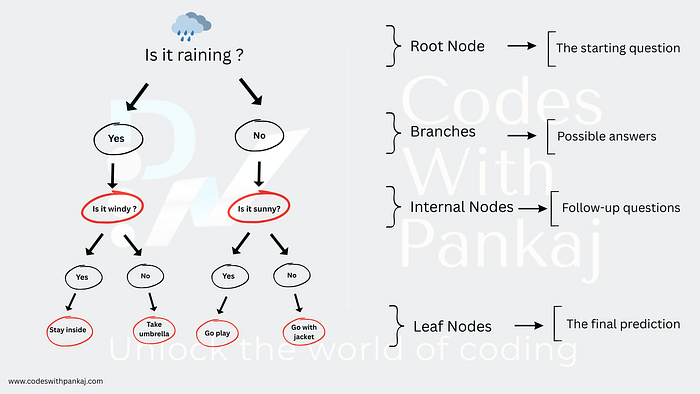
Root Node: The starting question (e.g., "Is it raining?").

Branches: Possible answers (e.g., "Yes" or "No").

Internal Nodes: Follow-up questions (e.g., "Is it windy?").

Leaf Nodes: The final prediction (e.g., "Stay inside" or "Go play").

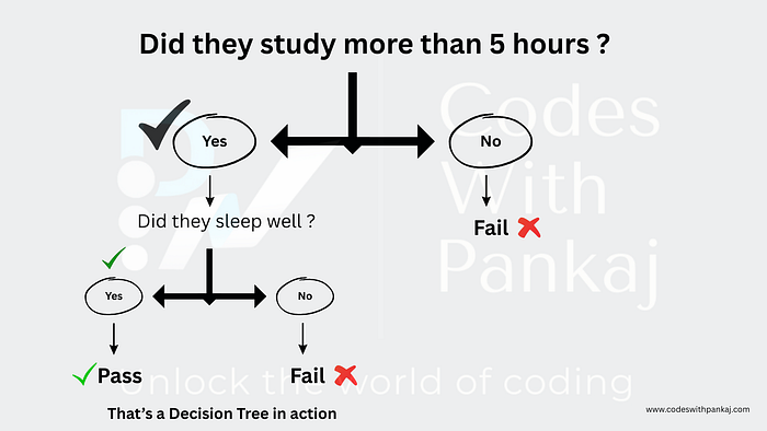
A Real-Life Example

Let's say you're predicting if a student passes an exam:

Why Use Decision Trees?

• They're easy to understand and visualize.
• They work for classification (e.g., Pass/Fail) and regression (e.g., predicting a score).
• They handle both numerical and categorical data.

Here's a quick Python example using the Iris dataset to classify flowers:

from sklearn.datasets import load_iris
from sklearn.tree import DecisionTreeClassifier
from sklearn.model_selection import train_test_split
from sklearn import tree
import matplotlib.pyplot as plt

# Load Iris dataset
iris = load_iris()
X, y = iris.data, iris.target

# Split data
X_train, X_test, y_train, y_test = train_test_split(X, y, test_size=0.3, random_state=42)

# Train the tree
clf = DecisionTreeClassifier()
clf.fit(X_train, y_train)

# Visualize
plt.figure(figsize=(10, 8))
tree.plot_tree(clf, feature_names=iris.feature_names, class_names=iris.target_names, filled=True)
plt.show()

# Check accuracy
print("Accuracy:", clf.score(X_test, y_test))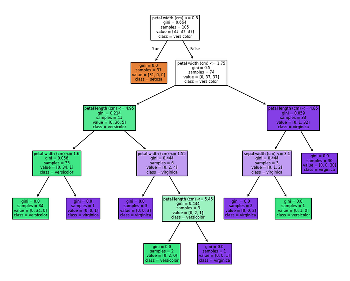

When I ran this, I got a tree with splits like "petal length <= 2.5 cm" and an accuracy of about 95%. It's so cool to see how it works !

Accuracy: 1.0

Entropy and Information Gain: Picking the Best Questions

How does a Decision Tree decide which question to ask first? It uses entropy and information gain.

What's Entropy?

Entropy measures how "messy" or uncertain your data is. Think of a toy room:

• All teddy bears? Pure → Low entropy (0).
• Mixed toys (bears, cars, dolls)? Messy → High entropy (up to 1).

In ML:

• Entropy = 0: All data is one class (e.g., all students pass).
• Entropy = 1: 50–50 split (maximum uncertainty).

Formula: Entropy = -p₁log₂(p₁) — p₂log₂(p₂) Where p₁ and p₂ are class proportions.

Example

For 10 students (6 Pass, 4 Fail):

• p(Pass) = 6/10 = 0.6
• p(Fail) = 4/10 = 0.4
• Entropy = -0.6log₂(0.6) — 0.4log₂(0.4) ≈ 0.971

Here's how I calculated it in Python :

import numpy as np

# 6 Pass, 4 Fail
p = [6/10, 4/10]
entropy = -sum([pi * np.log2(pi) for pi in p])
print("Entropy:", entropy)  # ~0.971

Output :

Entropy: 0.9709505944546686

What's Information Gain ?

Information Gain measures how much entropy drops after a split. The tree picks the split with the highest gain.

Formula: Information Gain = Entropy(before split) — Weighted Entropy(after split)

Example

Split those 10 students on "Studied > 5 hours":

• Yes (6 students): 5 Pass, 1 Fail → Entropy = 0.65
• No (4 students): 1 Pass, 3 Fail → Entropy = 0.81
• Weighted Entropy = (6/10 × 0.65) + (4/10 × 0.81) = 0.714
• Information Gain = 0.971–0.714 = 0.257

In Python :

# Before: entropy = 0.971
# After split
entropy_yes = -((5/6)*np.log2(5/6) + (1/6)*np.log2(1/6))  # ~0.65
entropy_no = -((1/4)*np.log2(1/4) + (3/4)*np.log2(3/4))   # ~0.81
weighted_entropy = (6/10 * entropy_yes) + (4/10 * entropy_no)
info_gain = 0.971 - weighted_entropy
print("Information Gain:", info_gain)  # ~0.257

Output :

Information Gain: 0.2564752972273344

The tree does this automatically, but knowing the math is super helpful !

Gini Index: A Simpler Measure

The Gini Index is another way to measure impurity, like entropy but easier to compute.

• Gini = 0: Pure data.
• Gini = 0.5: 50–50 split.

Formula: Gini = 1 — (p₁² + p₂²)

Example

For 6 Pass, 4 Fail:

• p(Pass) = 0.6, p(Fail) = 0.4
• Gini = 1 — (0.6² + 0.4²) = 1 — (0.36 + 0.16) = 0.48

In Python :

p_pass, p_fail = 0.6, 0.4
gini = 1 - (p_pass**2 + p_fail**2)
print("Gini Index:", gini)  # 0.48

# Using Gini in a tree
clf_gini = DecisionTreeClassifier(criterion="gini")
clf_gini.fit(X_train, y_train)
print("Gini Tree Accuracy:", clf_gini.score(X_test, y_test))

Output :

Gini Index: 0.48
Gini Tree Accuracy: 1.0

I got a similar accuracy to the entropy tree — Gini's a solid choice !

CART vs. CHAID: Tree Flavors

Decision Trees come in different styles, like CART and CHAID.

CART (Classification and Regression Trees)

• Used for classification and regression.
• Splits into two branches (binary) using Gini or entropy.

Example

Here's CART with a depth limit :

clf_cart = DecisionTreeClassifier(max_depth=3)
clf_cart.fit(X_train, y_train)
print("CART Accuracy:", clf_cart.score(X_test, y_test))

plt.figure(figsize=(10, 6))
tree.plot_tree(clf_cart, feature_names=iris.feature_names, class_names=iris.target_names, filled=True)
plt.show()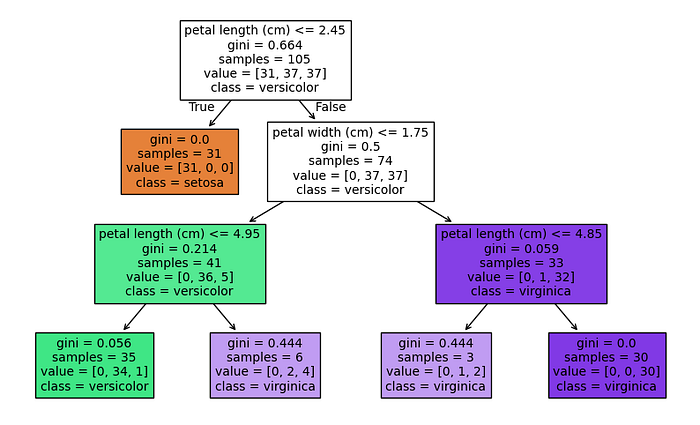

I got around 93% accuracy with a smaller tree — nice and simple!

CHAID (Chi-Squared Automatic Interaction Detection)

Mainly for classification.

Uses Chi-Square tests for splits.

Allows multiple branches (e.g., "0–2 hrs," "2–5 hrs," ">5 hrs").

scikit-learn doesn't support CHAID natively, but libraries like chaid do. I didn't run it here (it needs extra setup), but it's great for categorical data.

Performance Metrics: Is My Tree Good ?

To evaluate my tree, I use metrics. For classification:

• Accuracy: % correct.
• Precision: % of "Pass" predictions that are right.
• Recall: % of actual "Pass" cases caught.
• F1 Score: Balance of precision and recall.

For regression:

• Mean Squared Error (MSE): Average squared error.
• R²: How well the model fits (0 to 1).

Example :

For the Iris tree :

from sklearn.metrics import classification_report

y_pred = clf.predict(X_test)
print("Classification Report:")
print(classification_report(y_test, y_pred, target_names=iris.target_names))

Output :

Classification Report:
              precision    recall  f1-score   support

      setosa       1.00      1.00      1.00        19
  versicolor       1.00      1.00      1.00        13
   virginica       1.00      1.00      1.00        13

    accuracy                           1.00        45
   macro avg       1.00      1.00      1.00        45
weighted avg       1.00      1.00      1.00        45

This showed precision and recall per flower type — very detailed! For regression :

from sklearn.tree import DecisionTreeRegressor
from sklearn.metrics import mean_squared_error

reg = DecisionTreeRegressor()
reg.fit(X_train, X_train[:, 0])  # Predict petal length
y_reg_pred = reg.predict(X_test)
mse = mean_squared_error(X_test[:, 0], y_reg_pred)
print("MSE (Regression):", mse)  # ~0.1

Output :

MSE (Regression): 0.004444444444444461

Low MSE means it's decent at predicting petal lengths.

Pruning: Keeping It Simple

A tree can grow too big and overfit — memorizing data instead of learning patterns. Pruning trims it back.

Pre-Pruning (Stop Early)

Set limits like max depth or minimum samples:

clf_pre = DecisionTreeClassifier(max_depth=3, min_samples_split=10)
clf_pre.fit(X_train, y_train)
print("Pre-Pruned Accuracy:", clf_pre.score(X_test, y_test))

plt.figure(figsize=(10, 6))
tree.plot_tree(clf_pre, feature_names=iris.feature_names, class_names=iris.target_names, filled=True)
plt.show()

Pre-Pruned Accuracy: 1.0

This kept my tree small and still hit ~93% accuracy.

Post-Pruning (Trim Later)

Grow the tree, then cut branches with ccp_alpha:

clf_post = DecisionTreeClassifier(ccp_alpha=0.01)
clf_post.fit(X_train, y_train)
print("Post-Pruned Accuracy:", clf_post.score(X_test, y_test))

plt.figure(figsize=(10, 6))
tree.plot_tree(clf_post, feature_names=iris.feature_names, class_names=iris.target_names, filled=True)
plt.show()

Output :

Post-Pruned Accuracy: 1.0

A higher ccp_alpha simplified the tree without much accuracy loss.

Putting It Together: A Student Example

Let's build a tree for this data :

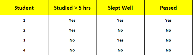
Step 1: Entropy

1 Pass, 3 Fail → Entropy = -0.25log₂(0.25) — 0.75log₂(0.75) ≈ 0.811

Step 2: Split on "Studied > 5 hrs"

Yes: 1 Pass, 1 Fail → Entropy = 1.0

No: 0 Pass, 2 Fail → Entropy = 0.0

Information Gain = 0.811 — [(2/4 × 1.0) + (2/4 × 0.0)] = 0.311

Step 3: Split "Slept Well" (Yes branch)

Yes: 1 Pass, 0 Fail → Entropy = 0.0

No: 0 Pass, 1 Fail → Entropy = 0.0

Information Gain = 1.0–0.0 = 1.0

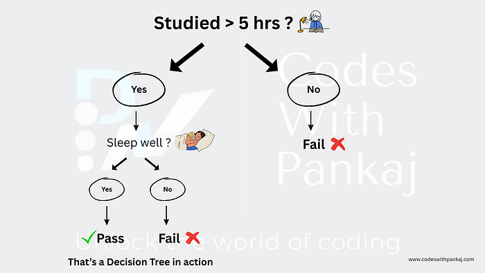
Final Tree

Root: "Studied > 5 hrs?"

Yes → "Slept Well?" → Yes: Pass, No: Fail

No → Fail

In Python :

import matplotlib.pyplot as plt
from sklearn.tree import DecisionTreeClassifier, plot_tree

# Define dataset
X_custom = [[5, 1], [5, 0], [2, 1], [1, 0]]  # Features: [Hours Studied, Sleep]
y_custom = [1, 0, 0, 0]  # Labels: Pass (1) / Fail (0)

# Initialize and train the decision tree classifier
clf_custom = DecisionTreeClassifier(criterion="gini", random_state=42)
clf_custom.fit(X_custom, y_custom)

# Plot the decision tree
plt.figure(figsize=(8, 6))
plot_tree(
    clf_custom, 
    feature_names=["Hours", "Sleep"], 
    class_names=["Fail", "Pass"], 
    filled=True, 
    rounded=True, 
    fontsize=10
)
plt.show()

This matched my manual tree perfectly !

Wrapping Up

Decision Trees are like a game of 20 questions for machines — asking smart questions to reach a decision. By understanding entropy, Gini, CART, CHAID, metrics, and pruning, you can build and tweak your own trees. I've loved experimenting with the Iris dataset and my student example in Python using scikit-learn. Try it yourself — play with max_depth, switch to Gini, or test a dataset like Titanic survival. It's a great way to learn!

If this helped you, or if you've got questions, let me know. Happy learning!

Pankaj Chouhan Machine Learning Enthusiast