A use-case study for Twitter users.

Over three decades, the Internet has grown from a small network of computers used by research scientists to communicate and exchange data to a technology that has penetrated almost every aspect of our day-to-day lives. Today, it is hard to imagine a life without online access for doing business, shopping, and socialising.

A technology that has connected humanity at a scale never before possible has also amplified some of our worst qualities. Online hate speech spreads virally across the globe with short and long term consequences for individuals and societies. These consequences are often difficult to measure and predict. Online social media websites and mobile apps have inadvertently become the platform for the spread and proliferation of hate speech.

What is online hate speech?

"Hate speech is a type of speech that takes place online (e.g., the Internet, online social media platforms) with the purpose to attack a person or a group on the basis of attributes such as race, religion, ethnic origin, sexual orientation, disability, or gender." [source]

A number of international institutions including the UN Human Rights Council and the Online Hate Prevention Institute are engaged in understanding the nature, proliferation, and prevention of online hate speech. Recent advances in machine learning have shown promising results to aid in these efforts, especially as a scalable automated system for early detection and prevention. Academic researchers are constantly improving machine learning systems for hate speech classification. Simultaneously, all major social media networks are deploying and constantly fine-tuning similar tools and systems.

Online hate speech is a complex subject. In this article we consider using machine learning to detect hateful users based on their activities on the Twitter social network. The problem and dataset were first published in [1]. The data are freely available for download from Kaggle here.

In what follows, we develop and compare two machine learning methods for classifying a small subset of Twitter's users as hateful, or normal (not hateful). First we employ a traditional machine learning method to train a classifier based on users' lexicons and social profiles. Next, we apply a state-of-the-art graph neural network (GNN) machine learning algorithm to solve the same problem, but now also considering the relationships between users.

If you wish to follow along, the Python code in a Jupyter Notebook can be found here.

Dataset

We demonstrate applying machine learning for online hate speech detection using a dataset of Twitter users and their activities on the social media network. The dataset was originally published by researchers from Universidade Federal de Minas Gerais, Brazil [1], and we use it without modification.

The data covers 100,368 Twitter users. For each user a number of activity-related features is available. Such features include the frequency of tweeting, the number of followers, the number of favourites, and the number of hashtags. Furthermore, an analysis of each user's lexicon derived from their last 200 tweets has yielded a large number of features with regards to language content. Stanford's Empath tool was used to analyse each user's lexicon with regards to categories such as love, violence, community, warmth, ridicule, independence, envy, and politics, and assign numeric values indicating the user's alignment with each category.

In total, we use 204 features to characterise each user in the dataset. For each user, we collect these features to form a 204-dimensional feature vector to be used as input to a machine learning model for classifying users as hateful or normal (see below).

The dataset also includes relationships between the users. A user is considered connected with another user if the former has re-tweeted the latter. This relationship structure gives rise to a different network than Twitter's network based on follower and followee relationships. The latter are hidden from us since users can elect to keep their network private. However, the retweet network is public as long as the original tweets are public.

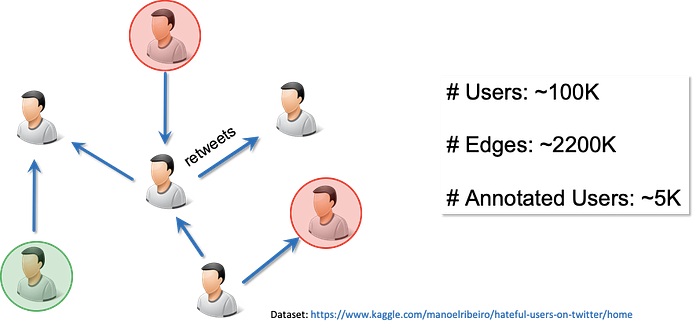
Finally, users are labeled as belonging to one of three categories: hateful, normal, and other. Out of ~100k (we use the symbol ~ to denote approximate numbers) users in the dataset, only ~5k have been manually annotated as hateful or normal; the remaining ~95k users belong to the other category, meaning they haven't been annotated. The authors in [1] describe in more detail the protocol guiding the data annotation process.

Figure 1 shows a graphical representation of the dataset. We show users annotated as hateful in red circles whereas we show users annotated as normal in green circles. Users labeled as other (not annotated) are left blank.

Hateful user classification using Machine Learning

Our objective is to train a binary classification model that can be used to classify users as hateful or normal. However, the dataset used to train the model presents two challenges.

Firstly, only a small subset of users is annotated as hateful or normal, with majority of users' labels unknown (other category). Secondly, the labeled data is highly imbalanced in terms of label distribution: out of the ~5k annotated users, only ~500 (~10%) have been annotated as hateful and the remaining as normal.

Semi-supervised machine learning methods can help us alleviate the small labelled sample issue by making use of both labelled and unlabelled data. We will consider such methods later in this article within the context of graph neural networks. To deal with class imbalance in the labelled training set, we calculate and use class weights; these weights are used in the model's loss function (that is optimised during model training) to penalise the model's mistakes in classifying users from the "minority" class (the class with fewer examples, in our case the hateful class of users) proportionally more than mistakes in classifying users from the "majority" class (the normal class of users).

Splitting the data into training and test sets

The following content demonstrates how to develop machine learning models using Python's data science tools. Here, we only include small but important code snippets while the full Python script can be accessed here.

The non-technical reader may safely skip to the sections titled "Comparison between models" and "Conclusion" at the end of the article.

As the model's objective is to classify users as hateful or normal, we use the annotated subset of users for training and evaluating the model. We begin by collecting all the feature vectors of the annotated users into the design matrix, annotated_user_features, such that the i-th row of the matrix corresponds to the feature vector of the i-th user. Next, we collect the user labels, hateful or normal, into the target vector annotated_user_targets.

We split this data into training and test sets using scikit-learn's train_test_split stratified sampling method, such that 15% of the annotated user data is selected for training and the remaining 85% for testing the trained classification model. In the code below we fix random_state for reproducibility of the split.

The statistics of our train and test sets are as follows;

Train normal: 664 hateful: 81

Test normal: 3763 hateful: 463

Given that the training data exhibit high class imbalance, we calculate class weights using scikit-learn's compute_class_weight method:

The class weights are 0.56 and 4.60 for known normal and hateful users respectively. The positive (hateful) class is underrepresented in the training data, and thus its examples will be given ~8x the weight of the negative (normal) class examples when calculating the loss function during model training. (Note that the minority class in a binary classification problem is typically regarded as "positive" by convention regardless of the actual meaning of the labels; this of course does not mean that being hateful is considered a positive trait.)

Evaluation metrics

In order to evaluate the performance and compare the trained classification models, we are going to consider the following three metrics (for a description of evaluation metrics for binary classifiers see here), evaluated on the held-out test set of annotated users:

• Accuracy
• Receiver Operating Characteristic (ROC) curve
• Area Under the ROC curve (AU-ROC)

Logistic regression model

Let's begin by training a logistic regression (LR) model to predict a normal or hateful label for a user. For computational convenience, we map the normal and hateful labels to the numeric values 0 and 1 respectively.

When training and evaluating this model, we will ignore users that are not annotated as either normal or hateful as well as the relationships between users due to lack of direct support for such information in logistic regression.

The train and test data are structured in tabular format as shown in Figure 2. The annotated users in the training set are shown using red and green circles. The feature vectors for each of the users are stacked vertically to create the design matrix, train_data. After training the logistic regression model, we can make predictions for the users in the held-out test set in order to measure the generalisation performance of the trained model.

We use scikit-learn's LogisticRegressionCV model that we train as follows:

Once the model is trained, we use it to predict probabilities to be hateful and normal for users in the test set:

Using the predicted probabilities for users in the test set, we can plot the ROC curve and calculate the accuracy and AU-ROC metrics. The accuracy on the test set is 85.9% and the AU-ROC is 0.81. A plot of the ROC curve can be seen in Figure 3.

Graph Neural Networks

In the specification and training of the logistic regression model, we ignored the ~95k users that have not been annotated as hateful or normal. Furthermore, we ignored the relationships between the users.

It is conceivable that a hateful user would take measures to avoid easy identification by, for example, being cautious not to use obviously hateful vocabulary. However, the same user might be comfortable retweeting other users' hateful tweets. This information is hidden in the relationships between users. The logistic regression model we employed above did not utilise these relationships.

Can we exploit the relationships between users, as well as the data about non-annotated users to improve the predictive performance of a machine learning model? And if so, what kind of machine learning model can we use and how?

One way to use the relationship data would be to do manual feature engineering introducing network-related features into the logistic regression model. Examples of such features include various centrality measures that quantify the positional importance of nodes in the graph. In fact, the dataset as published in [1] includes such engineered network-related features, but we have deliberately removed them from the data in order to demonstrate one of the core ideas in modern machine learning.

This idea—popularised by deep learning methods—is that it is possible to let the machine learning algorithm automatically learn suitable features that maximise model performance, thus avoiding the laborious process of manual feature engineering. (This automation of feature engineering, however, comes at a price of interpretability of the resulting model — a subject of another discussion.)

Guided by the above idea, we forgo feature engineering and tackle online hate speech classification using a state-of-the-art graph neural network algorithm (GNN). The GNN model jointly exploits user features and relationships between all users in the dataset, including those users that are not annotated. We expect that the GNN model using this additional information will outperform the baseline logistic regression model.

The article Knowing Your Neighbours: Machine Learning on Graphs provides an introductory yet comprehensive overview of graph machine learning.

The particular GNN algorithm we employ here was published in [3]. It is called Graph Sample and Aggregate (GraphSAGE) and builds on the insight that a prediction for a node should be based on the node's feature vector but also those of its neighbours, perhaps their neighbours as well, and so on. Using the example of classifying hateful users, our working assumption is that a hateful user is likely to be connected with other hateful users. The strength of this connection will depend on both the graph distance between the two users (the graph distance between the two user nodes) and their feature vectors.

GraphSAGE introduces a new type of graph convolutional neural network layer that propagates information from a node's neighbourhood while training a classifier. This new layer is summarised in Figure 4. As described in [3] such a layer "generates embeddings by sampling and aggregating features from a node's local neighbourhood."

An embedding is a latent representation of a node that can be used as input to a classification model, typically a fully connected neural network, such that we can train all the model parameters in an end-to-end fashion. We can stack several such layers in sequence to construct a deeper network that fuses information from larger network neighbourhoods. The number of GraphSAGE layers to use is problem specific and it should be tuned appropriately as a model hyperparameter.

Generally, graph neural network models can become computationally unwieldy for large graphs with high degree nodes. To avoid this, GraphSAGE employs a sampling scheme to limit the number of neighbours whose feature information is passed to the central node as shown in the "AGGREGATE" step in Figure 4.

Furthermore, GraphSAGE models learn functions that can be used to generate latent representations for nodes that were not present in the network during training. In consequence, GraphSAGE can suitably be used to make predictions in an inductive setting when only part of the graph is available at training time (while this is not the case for our working example, you can find such a demonstration in the Jupyter Notebook here.)

The open source StellarGraph Python library provides an easy to use implementation of the GraphSAGE algorithm. In this post, we will use StellarGraph to build and train a GraphSAGE model for predicting hateful Twitter users.

Earlier, we loaded the data into the Pandas DataFrame, annotated_user_features, and the corresponding target values into annotated_user_targets. We have also split our data into training and test sets, train_data and test_data respectively.

Now we load the graph structure into a NetworkX object using the following code, where the variable data_dir is pointing to the local storage system folder where the data is located:

Given the NetworkX object and the node features (for all ~100K user nodes) stored in a Pandas DataFrame, node_features, we create a StellarGraph object that prepares the data for machine learning using graph neural networks.

After loading the data we use it to specify the GraphSAGE model. In order to train the model, we first create a generator object that will feed data from the graph G to the model. The library includes generator objects specialised for all the graph neural network models it implements. For a GraphSAGE model, we must instantiate a GraphSAGENodeGenerator object specifying the StellarGraph object, G, to feed the data from, the mini-batch size for stochastic gradient descent training, and the number of random samples per hop to be sampled. The latter indicates the number of neighbours to sample (with replacement) for the "AGGREGATE" step in Figure 4, for each layer in the stack (the entire GraphSAGE model is a stack of K layers, where K is the length of the num_samples list).

Here the parameter num_samples is a list of length 2, hence we are implicitly specifying that for each node, we consider its 2-hop neighbourhood for feature aggregation and fusion; this entails the creation of a GraphSAGE model with two graph neural network layers of the type shown in Figure 4. For each node in the mini-batch (the root node), we sample 20 1-hop neighbours, and for each of those neighbours we sample 10 more neighbours, for a total of 20x10=200 nodes whose features are aggregated and fused with those of the root node.

The StellarGraph model is implemented as a stack of Keras layers, and is thus a Keras model. To feed the data into the model, we use the flow method of generator to create two iterators over the train and test sets of nodes. In the below code, we create the iterator train_gen over the training data by specifying the IDs and corresponding targets for the nodes in the train set. We then use the same generator object to create the test data iterator, test_gen, for feeding data to the model during model evaluation.

Finally, we create a StellarGraph GraphSAGE object comprising of a stack of two sample-and-aggregate layers as described above. We capture the input and output tensors of this model via the build method, and, finally, add a Keras Dense layer with a single output unit with sigmoid activation. The latter is the classification layer that outputs the probability of a user being hateful.

We wrap the resulting stack of layers into a Keras model, and compile it specifying the loss function to be optimised (binary cross entropy since we are solving a binary classification problem) and the optimiser to use for that (Adam optimiser [4]) with the initial learning rate of 0.005. We can also specify an optional list of evaluation metrics to keep track of during training; here we will be tracking the classification accuracy.

Finally, we train the model for 30 epochs as shown in the below code:

We can plot the values of the loss function (stored in the history variable) on the training and test data as shown in Figure 5.

Lastly, we visualise the node latent representations for the annotated users. We take the output activations of the first GraphSAGE layer as the node representations. These are shown in 2-D in Figure 6 where hateful users are shown in red and normal users in blue.

The node latent representations shown in Figure 6 indicate that the majority of hateful users tend to cluster together. However, some normal users are also in the same neighbourhood and these will be difficult to distinguish from hateful ones. Similarly, there are a small number of hateful users dispersed among normal users and these will also be difficult to classify correctly.

The GraphSAGE user classification model achieves an accuracy of 88.9% on the test data and an AU-ROC score of 0.88.

Comparison between models

Let's now compare the GraphSAGE and logistic regression models, to see whether using the additional information about unlabelled users and relationships between users actually helped to make a better user classifier.

The ROC curves for both models are drawn together in the Figure 7. The AU-ROC is 0.81 and 0.88 for the LR and GraphSAGE models respectively (larger numbers denote better performance). By this measure, we see that utilising relationship information in the machine learning model improves overall predictive performance.

When classifying users as hateful (positive class) or normal (negative class), it is important to minimise the number of false positives that is the number of normal users that are incorrectly classified as hateful. At the same time, we want to correctly classify as many hateful users as possible. We can achieve both of these goals by setting decision thresholds guided by the ROC curve.

Assuming that we are willing to tolerate a false positive rate of approximately 2%, the two models achieve true positive rates of 0.378 and 0.253 for GraphSAGE and LR respectively. We thus see that for a fixed false positive rate of 2%, the GraphSAGE model achieves a true positive rate that is 12% higher than the LR model. That is, we can correctly identify more hateful users for the same low number of misclassified normal users. We can conclude that by using the relationship information available in the data, as well as the unlabelled user information, the performance of a machine learning model on sparsely labeled datasets with underlying network structure is greatly improved.

Conclusion

In this article we considered the rise of online hate speech fuelled by the Internet's growth and asked the question; "Can graph machine learning identify hate speech in online social networks?"

Our technical analysis answers this question with a resounding; "Yes, but there is still plenty of room for improvement." We demonstrated that modern graph neural networks can help identify online hate speech at a much higher accuracy than traditional machine learning methods.

The Council on Foreign Relations recently published this article stating; "Violence attributed to online hate speech has increased worldwide." We have shown that graph machine learning is a suitably powerful weapon in the fight against online hate speech. Our results provide encouragement for additional research for online hate speech classification with larger network datasets and more complex graph neural network methods.

If you want to learn more about how to use state-of-the-art graph neural network models for predictive modelling, have a look at the StellarGraph graph machine learning library and the numerous accompanying demos.

This article was written in collaboration with Anna Leontjeva and Yuriy Tyshetskiy.

This work is supported by CSIRO's Data61, Australia's leading digital research network.

References

1. "Like Sheep Among Wolves": Characterizing Hateful Users on Twitter. M. H. Ribeiro, P. H. Calais, Y. A. Santos, V. A. F. Almeida, and W. Meira Jr. 2018.
2. Empath: Understanding Topic Signals in Large-Scale Text. E. Fast, B. Chen, M. S. Bernstein, Proceedings of the CHI Conference on Human Factors in Computing Systems, 2016.
3. Inductive Representation Learning on Large Graphs. W. L. Hamilton, R. Ying, and J. Leskovec, NeurIPS, 2017.
4. Adam: A Method for Stochastic Optimization, D. P. Kingma, and J. Ba, arXiv preprint arXiv:1412.6980, 2014.