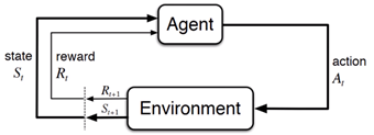
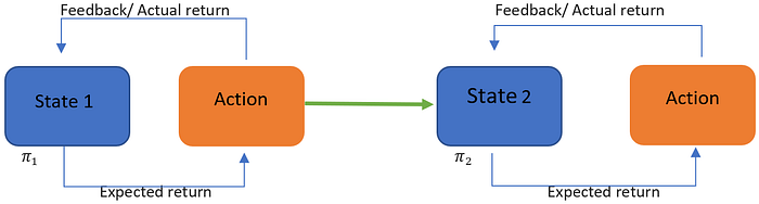
Reinforcement learning (RL) is a relatively new paradigm of Artificial intelligence and is becoming widely adopted for function optimization and control system problems. Reinforcement learning is considered one of the three main methods of Artificial Intelligence used currently (Alongside supervised learning and unsupervised learning); however, it is considered an unsupervised method. In the RL paradigm the AI (The Agent) continuously interprets and acts upon it's environment in the effort to maximize a defined goal [1]. The environment is presented to the Agent as a sequence of events, wherein the Agent attempts to take the action's which it believes will allow it the highest long-term reward.

This process simulates an actor critic model where the Agent acts upon its environment, then receives feedback on its action, such that the Agent's understanding of the environment can be further optimized. One of the most historically significant milestones of this form of AI was when a reinforcement learning algorithm defeated 9- dan professional Go board game player Lee Sedol [2]. This game was thought to be unlearnable by machine logic due to the game requiring players to use intuition, creativity and most importantly, an overarching long-term strategy. The extreme complexity of the game gave it the perception that the champion players were guided by incomprehensible intuition, gained from years and years of experience.

Whilst the Reinforcement learning framework has practically unlimited scope of use, in this article we will be focusing on its use in financial application. In these scenario's the Agent is interpreting the time series data as an environment it must navigate and must then employ its Q-learning method to optimize its decision making.

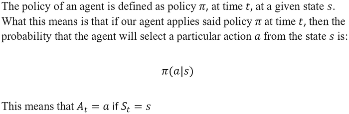
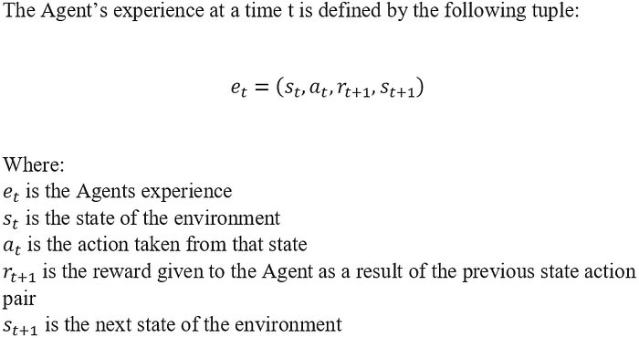
Throughout this paper the Q-learning AI shall be referred to as The Agent, and it is the Agents' goal to maximize a total reward, toward a certain goal, in a defined environment.

Markov decision process

This framework of an Agent maximizing a total net reward by attempting to take an optimal sequence of actions is known as a Markov decision process.

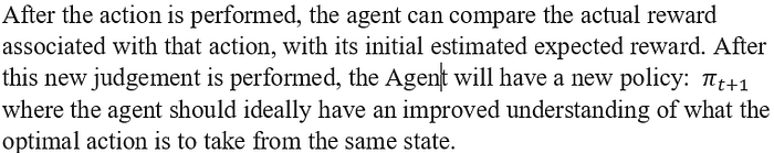
A Markov chain is a stochastic model, whereby the probabilities connecting a sequence of partially random events is examined [3]. A Markov chain depicts the associations between events in a sequence, which is critical for models used in financial analysis where underlying trends in data must be observed. In the Reinforcement paradigm the Agent is a Markovian decision-maker and is tasked with attempting to make optimal decisions based on its understanding of the data. This Agent's objective becomes a continuous process, where the Agent acts upon its environment then evaluates the outcome of their action, then takes this outcome into consideration in their next action.

See below a diagram of this Agent/ Action model. source: [4]

Markov decision process

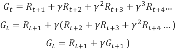
This Markov process is the formalized sequence of the Agent's actions, and can be represented as such:

In this Markov decision making process the transition between states is set to have a random element to it, where the likely states and rewards can be defined as a probability distribution.

This probability can be expressed as:

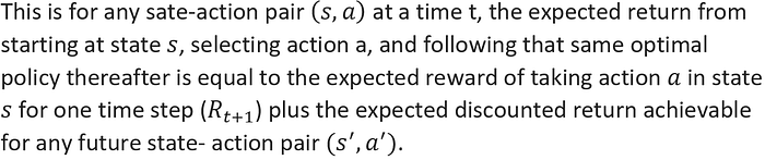
Expected return One key aspect of the Agents decision making process is the concept of expected return. Expected return refers to the reward that the Agent anticipates (expects) to receive from taking a particular action.

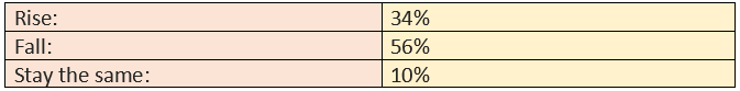
Q-learning Agents in most financial applications are used on Markovian sequence's, whilst attempting to maximize a particular defined goal. At each time step, the Agent must assess all possible next moves, from the current state (position) and must determine which action will achieve it the highest total return. To relate this to financial data, imagine a situation where the Agent is working with the opening/ close prices of a particular stock to devise a stock prediction policy. After a day ends our Agent may wish to predict what the stock price will do the following morning such that it can made the correct trade which would optimize profit/ mitigate loss. Our Agent would observe its current state and observe all of the possible actions which can be taken from that state. In this example there are three logical possible next states the price of the stock could take; It could rise in value, drop in value, or maintain its current value. From the Agents current state, it will evaluate which of these possibilities is most likely to occur. After a long computation by the Agent, it may for example decide that the probabilities associated with each possible change in state is:

In intra time step time series forecasting examples (like the above), the Agent does not need to think past the immediate short-term future. In other more advanced applications of reinforcement learning (such as portfolio optimization) a more long-term outlook of expected return is necessitated. For this reason, the concept of total return is used.

Total return

In order for the Agent to accurately perceive its expected return, it must be able to accurately predict the perceived total return. The total return is the long-term accumulation of the rewards achieved by the Agent across its action making lifespan. To relate this back to a stock price prediction example, the reward given to the Agent upon each action would be feedback as to how close its estimation was to the actual outcome. The Agent would be rewarded positively for accurate prediction and would be penalized for inaccuracy. Ultimately once the Agent has completed its lifespan, the total return the Agent has achieved is the accumulated rewards achieved by the Agent at timestep. This total return can be perceived by the Agent in a pre-emptive manner in regards a particular action (expected return), or retrospectively (total cumulative reward). It is our Agents' goal to maximize not just the return at each time step, but the total return over the whole process.

The total return of an Agent across its entire lifespan can be expressed like this:

Where T is the final time step.

As the Agent is iteratively exposed to the training data, it will begin creating policy's and performing actions which allow it greater total return. This simulates teaching the Agent about the environment, where the Agent continuously optimizes its decision-making policy associated with the environment.

Discounted return In a simplistic approach the concept of total return would be sufficient to drive sequential decision making, however a method named discounted return needs is incorporated to accommodate for more complex decision making.

Whilst the immediate reward of an action may be a good indicator as to the return of that particular action, it does not account for the future influence that action may have. This brings us to the concept of discounted return, which is a value which changes the rate of which future rewards are considered in present decision making. For example, in a simple intraday forecasting model the perception of future rewards is not necessitated as much, however many reinforcement learning applications centered around portfolio optimization and board game strategy have much greater need for this long-term perspective.

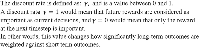
In general, reinforcement learning Agents place greater weighting on short term outcomes, as the rewards are considered to be more valuable when they are received sooner rather than later. This concept is similar to the financial concept of the time value of money, and in Reinforcement learning tasks such as portfolio optimization the relevance is clear.

This discounted return is what our Agent relies upon to evaluate the expected return from a certain action, and can be expressed as:

[1]

Further to this discounted return rate, the relationship of how the returns at successful timesteps are related can be defined as this equation:

Policies and values

Policy Due to this inevitability of random events occurring, our Agent is not expected to have perfect decision making. Rather, our Agent must develop an optimal policy, where the Agent must develop the best general set of actions which can be taken from each given state. This optimal policy is the policy which the Agent learns from the sample data, which it considers to be the policy that allows the Agent to produce the set of actions which optimizes its total return. Due to aspects such as arbitrage forces and noise in the data, our Agent must understand what to interpret literally and what to ignore in its decision-making process [5]. In the context of financial time series data, the Agent must learn the underlying trend's present in the data, as some changes in the data may be due to random factors.

For example, if an Agent where to analyze financial data for the year 2020, it would observe very large drawdowns across the world in March due to the COVID-19 pandemic. It is important that our Agent does not get the impression that that sharp downturn was for example a cyclical downturn due to steep economic growth in most countries over the last few years. The COVID-19 pandemic downturn did in fact happen when many economists were flagging an imminent global downturn, and an Agent taking the historical data too literally may interpret the downturn as being inevitability cyclical. For our Agent to develop its best policy it must understand what historical events in the data were expected and what was unexpected, so that it can iteratively improve the accuracy of its decision-making policy as it gets trained.

The optimal policy learnt by an Agent will be product of the features both learnt and forgotten in order to establish its perception of what most accurately represents the underlying function in the historical data. This optimal policy is significant when the Agent is not expected to achieve perfect decision making.

To explain this, I would like to compare a significant difficulty AI faced when trying to learn the board game go, versus AI's ability to play simpler games such as chess. The Go board game has significantly more places to move then a chess board, with each individual place on the board adding an exponential amount of possible additional states. Whereas in chess, where an AI model is able to perceive and compute every possible combination of moves in a game then tend toward the most perfect strategy, in imperfect decision making the Agent must devise the best possible strategy from its imperfect decision-making capabilities. It is Reinforcement learning's ability to create an optimal policy in an imperfect decision making process that has made it so revered.

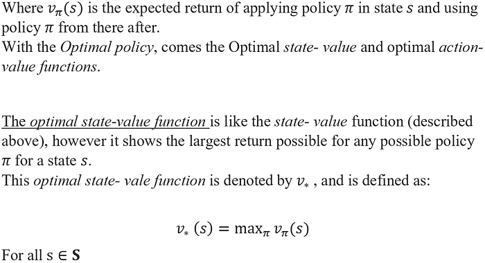
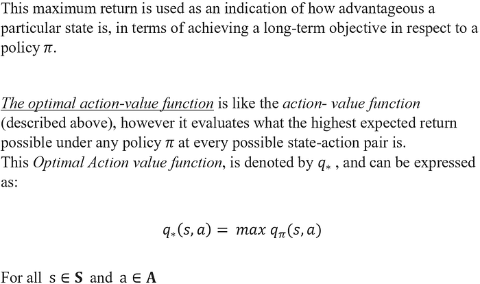
Value Value functions are used to estimate how much benefit "value" there is in being at a particular state, or how good it is for a certain action to be taken from a particular state. The former is referred to as the state-value function, and the latter is the action-value function. This value is perceived as an expected return, where the Agent evaluates how advantageous a position, or a particular decision will be in maximizing their total objective.

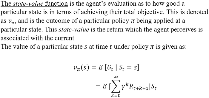
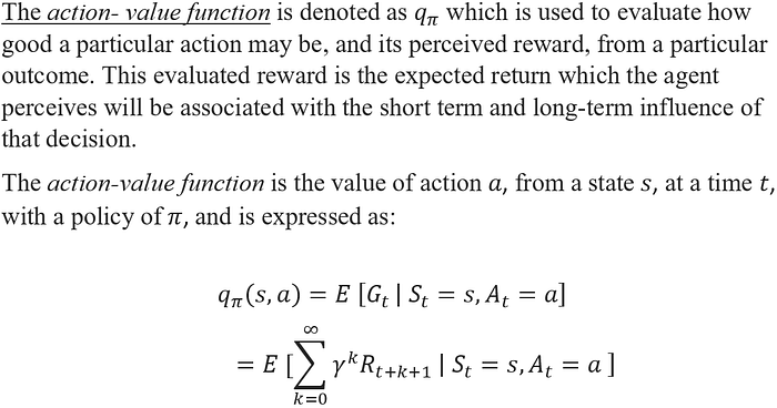
These concepts together give our Agent perspective of how valuable a particular state or decision is. For example, if a reinforcement learning Agent was playing a chess game, it would evaluate at each move; how valuable its current state is, and how valuable (to maximize a reward) each possible action may be from that state. The value of which an Agent perceives in a particular situation is unique to that Agent and the policy which it has learnt up until that point.

Optimal policy

The Agent's ultimate objective is to devise an optimal policy which allows it a general understanding, such that it can predict future events and optimize its goal. This optimal policy is the policy which the Agent believes will achieve it the highest long term expected return. This optimal policy can be updated at any point, and the Agent will update its optimal policy at any point where it believes a new policy will provide the Agent with a greater total reward for all future states.

Establishing the optimal policy (Q-learning)

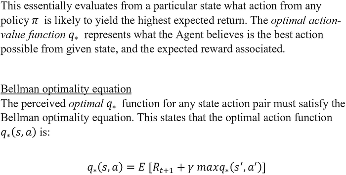
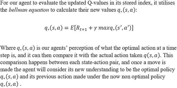
Q-learning is a method of establishing an optimal policy in a Markov decision process [6]. Q-learning is a technique that enables sequential decision making and is an unsupervised AI method capable of learning unlabeled data. The policy is considered optimal when the expected return over all the time steps is the maximum achievable. For this total expected return to be calculated, the optimal action must be established for each state-action pair (actions with the largest Q-value), which will form our Agent's optimal decision-making sequence.

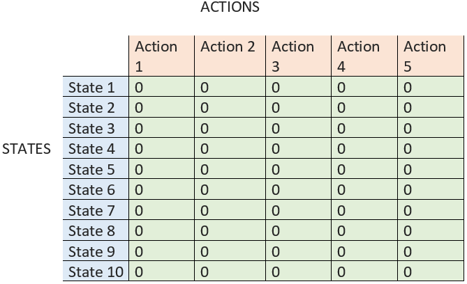
The optimal policy must be learnt by our Agent and is done so by iteratively updating its understanding of optimal actions at each time step such that eventually it develops a deep understanding. A unique element to Q-learning is that the optimal actions learnt by the Agent are stored in an index known as the Q-table.

See below for the general form a Q-table can take:

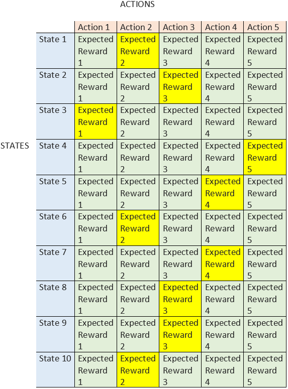
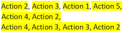
Total action choices from states 1- 10:

Our agent will iteratively run through the data selecting actions and learning from their outcomes, until it is able to produce what it believes it the best possible move for each state action pair.

The Agent will perceive actions and their associated expected rewards with a mapping like this, where it will select actions based on what the perceived optimal action is. The Q-table will eventually hold each ideal action for each state-action pair, and the values are iteratively updated by our Agent as it develops its knowledge of the data.

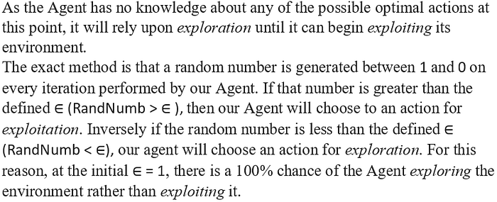
Exploration/ exploitation In order for the Agent to learn what the optimal action is for each state action pair, it must begin with very little knowledge of the environment and then form its own perception of the environment's rules. For our Agent to do this effectively, it must know when to explore the environment and when to exploit it.

Exploration Exploration is when a random action is selected, in an effort to learn from the environment. This is done when the Agent wishes to learn more about the rewards associated with actions. When the Agent is first introduced to the data it initially has no understanding of it and must learn by choosing random exploration actions and comprehending the rewards associated with them.

Exploitation Exploitation is when a particular action is made which uses the policy to take an action which it believes has the optimal Q-value and will return the maximum reward [7]. This is a deliberate action taken by the Agent with a desired outcome in mind, unlike an exploration move, where the action is taken for the purpose of learning from the outcome.

Although exploitation has obvious relevance at the start of our Agents journey, it is also imperative that exploration actions are done even when the Agent has a good sense of the environment. It is important so that the Agent does not fall into any non-optimal habits in its policy. For example, if the Agent learns one move which is semi optimal in the short term, it may continuously select that action and receive the same semi optimal short-term goal. If this game had the potential for an action which bore significant long-term rewards, the Agent may neglect to explore the environment sufficiently to discover it, as it may fall into the habit of relying upon the short term semi optimal reward.

Updating the Q-value Upon every action taken by our Agent it must reassess its understanding of the ideal Q-values and optimal policy. This retrospective judgment of the previous action, and reassessment of the policy, is based off judging the difference between what the optimal action should have been, and what the action taken actually was. The previous decision could be deemed optimal; however, it is the retrospective comparison is what drives our Agent's perception of how optimal a prior decision and its policy used was.

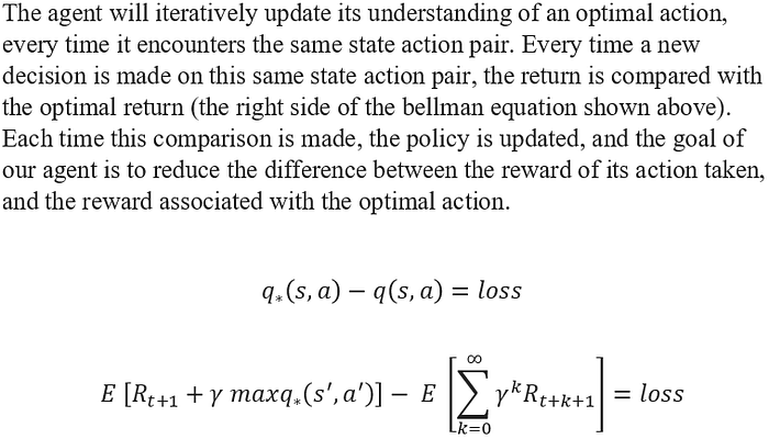
As we can see, the final learnt Q-value is a combination of the old known Q-value and the Recent learned Q-value.

Deep- Q Networks (DQN's)

Whilst the vanilla reinforcement learning approach is highly effective in creating an optimal policy in a Markov decision process, systems must often incorporate a most sophisticated method for value approximation than simple value iteration. Rather than relying on value iteration to iteratively update Q-vales, by incorporating neural networks for this value approximation, it allows the Q-learning Agent a much more sophisticated and deep ability to establish an optimal policy. This formulates a Deep Q-Network, which are an extension of the standard Q-learning paradigm and are considered an extremely capable extension of the unsupervised machine learning Agent. By incorporating Neural Network approximators into the Q-learning paradigm, the Agent is able to solve for the optimal Q-value at each state action pair, and thus the optimal function. The neural network incorporation for value estimation allows for accurate policy estimation in large complex environments. See below for a general diagram of a DQN policy network.

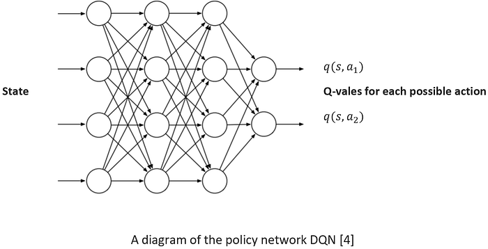
A diagram of the policy network DQN [4]

On the left-hand side, the input into the network is the state of the Agent. Upon Assessing this state, the Agent will approximate the optimal action which the Agent can take from that state (optimal Q-Value).

On the right-hand side of the network is the Q-value for each possible action which can be taken from that state. By utilizing the Bellman Equation (listed above), the network will evaluate each of the possible actions it can take (and their corresponding Q-values) and will update its perceived most optimal value every time it encounters a move with a higher Q-value for a particular state-action pair. The Agent will select the action which it calculates has the highest probability of achieving the highest reward (in exploitation).

Once the Agent takes the selected action it can assess the immediate reward associated with that action. Upon receiving this retrospective reward signal, the Agent calculates the loss associated with that action compared to the retrospective ideal action. Once the Agent evaluates the loss function associated with its previous decision, the weights in the network are updated via stochastic gradient descent and backpropagation. This simulates the Agent learning from its previous action and reassessing its perception of its optimal policy.

Deep-Q training

During the training process associated with a deep- Q architecture, the techniques of experience replay and Replay memory are used in training our Agent [4].

The DQN Agent relies upon the technique of experience replay to store its experiences in an index known as Replay memory. Replay memory is a dataset which stores information about the Agents recent experiences, so that the Agent can sample from it to train the network. The size of replay memory will generally be a finite number, such that the Agent will forget about memories once they have been stored past this finite number.

The target network

The above figure diagram shows the policy network layout for determining which action has the highest Q-value from that state. This neural network is effective, however an additional one must be incorporated on top of it known as the target network. The target network is similar to policy network shown above, and it actually copies all weights in the policy network, however the network is used to predict the optimal Q-value (optimal target) which it thinks is associated with that same state action pair. Whereby in the action network where the optimal action is predicted, the target network is used to predict what the Optimal Q-value (target value) is for that same state action pair.

This target network is important as Q-learning is an unsupervised method of AI, thus the targets are not given to the Agent. This means it must have a continuous method for approximating what the target Q-values are for each state action pair.

Performance in financial Application

For time series data to be used in Q-learning, it must be processed. One of the underlying assumptions of Q-learning is that the input data is stationary. Stationary data is data whereby the mean does not change, this means that for any trending time series data it is not initially stationary. There are many approaches to achieving stationarity in the data, however differencing seems to be the most widely employed method currently.

By transforming the data into stationary, the result is a set of repeating states which the Agent can interpret and predict. Whilst these states can be produced by simple differencing, it is also very common when implementing time series data to predict even simpler states such as; the rise, fall, or plateau of a particular stock. The more states the Agent is attempting to choose from the less accurate the Agent is likely to be, however reducing possible states may oversimplify the model more than wanted.

See below for the performance of Q-learning in predicting financial time series data:

Bibliography

[1] R. S. Sutton and A. G. Barto, Reinforcement learning: An introduction. MIT press, 2018.

[2] C.-S. Lee et al., "Human vs. computer go: Review and prospect [discussion forum]," IEEE Computational Intelligence Magazine, vol. 11, no. 3, pp. 67–72, 2016.

[3] C. J. Geyer, "Practical markov chain monte carlo," Statistical science, pp. 473–483, 1992.

[4] A. M. Andrew, "REINFORCEMENT LEARNING: AN INTRODUCTION by Richard S. Sutton and Andrew G. Barto, Adaptive Computation and Machine Learning series, MIT Press (Bradford Book), Cambridge, Mass., 1998, xviii+ 322 pp, ISBN 0–262–19398–1,(hardback,£ 31.95)," Robotica, vol. 17, no. 2, pp. 229–235, 1999.

[5] M. F. Dixon, I. Halperin, and P. Bilokon, Machine Learning in Finance. Springer, 2020.

[6] C. J. Watkins and P. Dayan, "Q-learning," Machine learning, vol. 8, no. 3–4, pp. 279–292, 1992.

[7] R. Dearden, N. Friedman, and S. Russell, "Bayesian Q-learning," in Aaai/iaai, 1998, pp. 761–768.

[8] J. Lee, "Stock price prediction using reinforcement learning," ISIE 2001. 2001 IEEE International Symposium on Industrial Electronics Proceedings (Cat. №01TH8570), vol. 1, pp. 690–695 vol.1, 2001.

[9] P. C. Pendharkar and P. Cusatis, "Trading financial indices with reinforcement learning agents," Expert Systems with Applications, vol. 103, pp. 1–13, 2018.

[10] J. Carapuço, R. Neves, and N. Horta, "Reinforcement learning applied to Forex trading," Applied Soft Computing, vol. 73, pp. 783–794, 2018.

[11] N. Kanwar, "Deep Reinforcement Learning-based Portfolio Management," 2019.

[12] S. Sornmayura, "Robust forex trading with deep q network (dqn)," ABAC Journal, vol. 39, no. 1, 2019.

[13] O. Jangmin, J. Lee, J. W. Lee, and B.-T. Zhang, "Adaptive stock trading with dynamic asset allocation using reinforcement learning," Information Sciences, vol. 176, no. 15, pp. 2121–2147, 2006.