


Introduction
Power calculation is a necessary step in the design of experiments. It plays a critical role in the estimation of the sample size needed to detect a given effect, or, the minimum detect effect we may expect given a fixed sample size and other design parameters. In this article, I will introduce both analytical and simulation methods with examples in R.
The power of the design is the probability that, for a given effect size and a given statistical significance level, we will be able to reject the hypothesis of zero effect (Duflo et al. 2007). In other words, power is the probability of correctly rejecting the null hypothesis when a treatment effect exists (i.e., when the null hypothesis is false).
Components of Basic Power Calculation
I think the simplest way to understand the components of power calculation is using the closed-form formula for Minimum detectable effect (MDE):

- MDE: the smallest effect size we can distinguish from zero given our design parameters, the smaller of the effect size we can detect, the more statistical power we have.
- P: the proportion of the sample allocated to the treatment group.
- Significance level or size of a test(α): The probability type I error or false positive: rejecting the null hypothesis of no effect when the null hypothesis is true (i.e., concluding the treatment had an effect when it did not). It is typically set at 5%.
- Power (1-κ): κ is the probability of type II error or false negative: failing to reject null hypothesis when null hypothesis is false (i.e., failing to detect the effect when there is one).Typically set at 0.8.
- N: sample size
- σ: standard deviation of the outcome variable
There are several relationship we can learn from the equation:
- It also implicitly defines the sample size N required to achieve a desired level of power.
- Increasing sample size decreases MDE and increases power.
- Decreasing outcome variance (less variation in the underlying population) decreases MDE and increases power increases.
- There is a trade-off between power and size. When α increases, the MDE increases for a given level of power. There is trade-off between the probability of falsely concluding that the treatment has an effect when it does not and the probability of falsely concluding that it has no effect when it does.
- An equal split between treatment arms typically maximizes the power.
Next, we put those things into tests in R:
Running the code above will return the results below. It shows that deviating from the 50/50 treatment/control allocation increases MDE, and increasing sample size greatly decreases MDE, as we expected. I use runif() to create random variables drawn from uniform distribution, we can see that the std. deviation is unchanged when I use the same runif(100,0,5)to produce 100 random uniform draws from a uniform distribution that goes from 0 to 5, decreases with runif(1000,0,1)and increases with runif(10,0,8).When the variance decreases, the MDE decreases.
It also shows that, if we want to be able to detect an effect size≥0.25 with 80% power (80% of chance detecting the effect), given the outcome variable distribution, we need a sample size of 1000. If we only collected a sample of 100 units, we would not be able to distinguish an effect<0.8 from zero even if it is.
baseline: sample size: 100 std dev: 1.424976 MDE: 0.8023922
decrease treatment allocation to 20%: sample size: 100 std dev: 1.424976 MDE is bigger: 1.00299
increase treatment allocation to 70%: sample size: 100 std dev: 1.424976 MDE is bigger: 1.00299
decrease outcome variable variance: sample size: 100 std dev: 0.2874839 MDE is smaller: 0.1618798
increase outcome variable variance: sample size: 100 std dev: 2.35792 MDE is bigger: 1.327725
increase sample size: sample size: 1000 std dev: 1.424976 MDE is smaller: 0.2526117
decrease sample size: sample size: 10 std dev: 1.424976 MDE is bigger: 2.67033
Power Calculation using Simulation
The basic idea of a simulated power analysis is to construct some data either through simulation or existing historical data, pre-set the sample size and effect size (or any other parameters we would like to test), use an analytical method such as regression, run it a bunch of times so wen can see the sampling variation of the power.
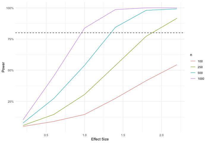
The code below does the following: I assumed a list of sample size and effect size I would like to try, created random variable X from a uniform distribution and Y by adding additional random noise to effect*X, ran a simple linear regression and got the probability of correctly rejecting the null when null is false at a significance level of 5% , then I ran the same process 500 times to get the sampling variation of the statistical power from which I calculated the mean of it.
At the end of the program, I created the graph below that shows the minimal detectable size or smallest sample size for a given power level such as 80% marked by the dashed line. For example, to be able to detect an effect size of 1.0–1.5 with 80% power (80% of the time we can find such effect) , we'd need a sample size at least 500. Given a sample size of 250, we'd only be able to detect effects > ~1.8. In other words we need an effect larger than 1.8 to have an 80% chance of finding a significant result. If we don't think the effect is actually likely to be that large, we need to tweak our experiment design — increase the sample, use a more precise estimation method.
Lastly, here is a list of some good references for power analysis:
Athey, Susan, and Guido Imbens. 2017. "The Econometrics of Randomized Experiments." Handbook of Field Experiments, 73–140.
Bloom, Howard S. "The core analytics of randomized experiments for social research." The SAGE handbook of social research methods (2008): 115–133.
Duflo, Esther, Rachel Glennerster, and Michael Kremer. 2007. "Using Randomization in Development Economics Research: A Toolkit." Handbook of Development Economics, 3895–3962.
Gelman, Andrew, and Jennifer Hill. 2006. "Sample size and power calculations" in Data Analysis Using Regression and Multilevel/Hierarchical Models, 437–454. Cambridge University Press: Cambridge, UK. http://www.stat.columbia.edu/gelman/stuff_for_blog/chap20.pdf.
List, John A., Azeem M. Shaikh, and Yang Xu. 2019. "Multiple hypothesis testing in experimental economics." Experimental Economics, 22: 773–793.
McConnell, Brendon, and Marcos Vera-Hernandez. 2015. "Going beyond simple sample size calculations: a practitioner's guide." IFS Working Paper W15/17. https://ifs.org.uk/publications/7844.
Özler, Berk. "When should you assign more units to a study arm?" World Bank Development Impact (blog), June 21, 2021. https://blogs.worldbank.org/impactevaluations/when-should-you-assign-more-units-study-arm?CID=WBW_AL_BlogNotification_EN_EXT. Last accessed August 3, 2021.
Nick Huntington-Klein. "Simulation for Power Analysis", December, 2021. https://nickch-k.github.io/EconometricsSlides/Week_08/Power_Simulations.html