Introduction

JAX, developed by Google, has gained significant traction in the machine learning and numerical computing communities. It is a high-performance library for numerical computation that combines the flexibility of NumPy with the scalability of machine learning frameworks like TensorFlow and PyTorch. What sets JAX apart is its ability to compute gradients and its efficient compatibility with GPUs and TPUs. In this guide, we'll explore JAX's core concepts, explore its unique features, and walk through practical examples.

What is JAX?

JAX can be summarized as a library for numerical computation that supports automatic differentiation and runs efficiently on accelerators like GPUs and TPUs. At its core, JAX provides:

1. NumPy Compatibility
2. Automatic Differentiation
3. Composable Transformations

JAX was designed to bridge the gap between research flexibility and production-level efficiency. Unlike other libraries, it integrates with NumPy seamlessly while offering transformative features that elevate numerical computation to the next level.

Setting Up JAX

Before diving into code, ensure you have JAX installed. JAX installation can vary depending on whether you use a CPU or GPU/TPU. For most cases, you can install JAX using the following commands:

!pip install jax[jaxlib]  # For CPU
!pip install jax[jaxlib] -f https://storage.googleapis.com/jax-releases/jax_cuda_releases.html  # For GP!U

Ensure that your system's CUDA version matches the JAX library version if you are leveraging GPUs for computation. The official JAX documentation is a great resource for troubleshooting installation issues.

Core Concepts in JAX

1. NumPy on Steroids

JAX's jax. numpy module provides NumPy-compatible functionality but with added support for hardware acceleration. Let's explore its capabilities with a simple example:

import jax.numpy as jnp
# Example: Element-wise operations
x = jnp.array([1.0, 2.0, 3.0])
y = jnp.array([4.0, 5.0, 6.0])
result = x + y
print(result)  # Output: [5. 7. 9.]

Output:

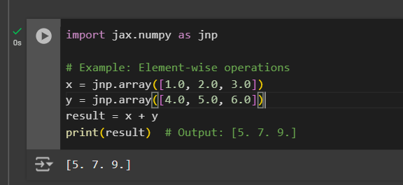
The key difference between JAX's arrays (DeviceArray) and NumPy's arrays is that JAX arrays are immutable. This immutability ensures thread safety and avoids unintended side effects in parallel computations. JAX also supports broadcasting, slicing, and other operations, just like NumPy.

2. Automatic Differentiation

One of JAX's standout features is its grad function, which enables automatic differentiation. This is particularly valuable for optimization tasks in machine learning. For instance, suppose we have a simple quadratic function:

from jax import grad
def simple_function(x):
    return x**2 + 3*x + 2
grad_fn = grad(simple_function)
print(grad_fn(2.0))  # Output: Gradient at x=2.0 (7.0)

Output:

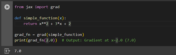
Here, the derivative of the function at is.

JAX computes gradients using reverse-mode differentiation, which is efficient for functions with a single scalar output, such as loss functions in machine learning.

3. Just-In-Time Compilation (JIT)

Just-In-Time (JIT) compilation is a powerful feature of JAX that optimizes performance by compiling Python functions into efficient machine code. This can significantly accelerate computation-heavy tasks.

from jax import jit
@jit
def compute_sum(x, y):
    return jnp.dot(x, y)
x = jnp.ones((1000, 1000))
y = jnp.ones((1000, 1000))
result = compute_sum(x, y)
print(result)

Output:

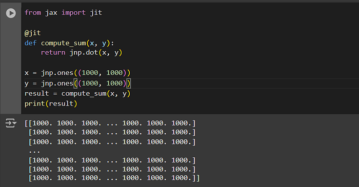
JIT transforms your Python function into a highly optimized version. Keep in mind that the first invocation may take longer due to the compilation overhead, but subsequent calls will be much faster.

4. Vectorization (vmap)

Vectorization allows you to apply functions over batches of data efficiently without the need for explicit loops. JAX provides vmap to achieve this seamlessly.

from jax import vmap
def square(x):
    return x**2
batched_square = vmap(square)
data = jnp.array([1.0, 2.0, 3.0, 4.0])
print(batched_square(data))

Output:

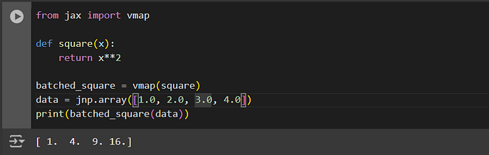
vmap eliminates the need for manual batching, enabling cleaner and more efficient code.

Practical Guide

Example 1: Gradient Descent Optimization

Gradient descent is a fundamental algorithm in machine learning for optimizing functions. Let's implement gradient descent using JAX to minimize a quadratic loss function.

from jax import grad
import jax.numpy as jnp
def loss_fn(x):
    return (x - 3)**2
# Gradient of the loss function
grad_loss = grad(loss_fn)
# Gradient descent loop
x = 0.0  # Initial value
learning_rate = 0.1
for i in range(20):
    grad_val = grad_loss(x)
    x -= learning_rate * grad_val
    print(f"Step {i+1}: x = {x:.4f}, loss = {loss_fn(x):.4f}")

Output :

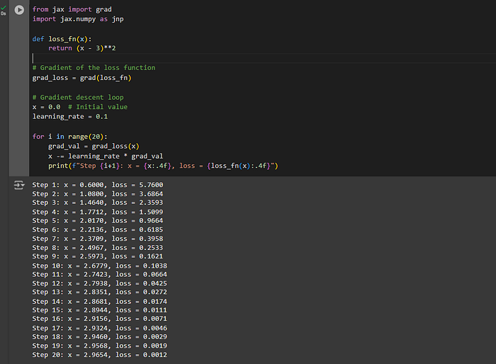
In this example, the gradient of the loss function is computed iteratively to update. As the algorithm progresses, converges to the minimum value of 3, and the loss approaches zero.

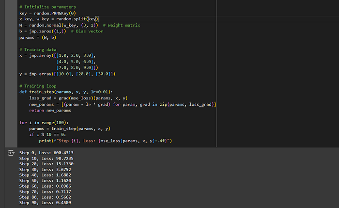
Example 2: Neural Network Training

Using JAX, we can define and train a simple single-layer neural network. This example demonstrates how to initialize parameters, compute the loss, and update weights using gradients.

from jax import random
import jax.numpy as jnp
from jax import grad, jit, vmap
# Define a single-layer neural network
def neural_network(params, x):
    W, b = params
    return jnp.dot(x, W) + b
# Loss function
def mse_loss(params, x, y):
    predictions = neural_network(params, x)
    return jnp.mean((predictions - y)**2)
# Initialize parameters
key = random.PRNGKey(0)
x_key, w_key = random.split(key)
W = random.normal(w_key, (3, 1))  # Weight matrix
b = jnp.zeros((1,))  # Bias vector
params = (W, b)
# Training data
x = jnp.array([[1.0, 2.0, 3.0],
               [4.0, 5.0, 6.0],
               [7.0, 8.0, 9.0]])
y = jnp.array([[10.0], [20.0], [30.0]])
# Training loop
def train_step(params, x, y, lr=0.01):
    loss_grad = grad(mse_loss)(params, x, y)
    new_params = [(param - lr * grad) for param, grad in zip(params, loss_grad)]
    return new_params
for i in range(100):
    params = train_step(params, x, y)
    if i % 10 == 0:
        print(f"Step {i}, Loss: {mse_loss(params, x, y):.4f}")

Output :

You can access the code here

Key Advantages

1. NumPy Compatibility: JAX serves as a drop-in replacement for NumPy with added support for GPU and TPU acceleration.

2. Automatic Differentiation: It enables efficient computation of gradients, critical for optimization and machine learning tasks.

3. High Performance: JAX supports Just-In-Time (JIT) compilation, dramatically improving computational speed for complex functions.

4. Scalability: With tools like vmap and pmap, JAX allows seamless vectorization and parallelization for large-scale computations.

5. Immutable Data Structures: Ensures thread safety and avoids side effects, ideal for parallel computing.

6. Flexibility: JAX integrates easily into research workflows and supports experimentation with new models and algorithms.

7. Open-Source and Actively Developed: Backed by Google and the open-source community, JAX is continuously improved and updated.

Conclusion

JAX has proven to be a transformative library for numerical computation and machine learning, blending the flexibility of NumPy with powerful features like automatic differentiation, JIT compilation, and vectorization. It empowers researchers and developers to perform high-performance computations effortlessly, leveraging hardware accelerators like GPUs and TPUs. Whether you're prototyping algorithms, training neural networks, or optimizing complex systems, JAX provides a robust and scalable framework.

Key Takeaways

1. JAX simplifies complex numerical tasks with its efficient API.
2. Its support for hardware acceleration ensures scalability and speed.
3. Tools like grad, jit, and vmap make it versatile for various domains.
4. While it has a learning curve, the effort is well-rewarded with unmatched performance and flexibility.