How to Use Python in R with Reticulate and Conda

Set up Reticulate in two simple steps and get the most out of R and Python libraries

Denisa Blackwood

Save The Data

· ~6 min read · October 24, 2021 (Updated: January 4, 2022) · Free: No

We've all been there once or twice: you know the perfect Python function and you're itching to use it, except you can't. You're stuck with R till the end of days. Or so you thought. No more! Perform this easy setup with Reticulate and Conda for your project and never make do without Python again.

This method is for you if you use the RStudio IDE (version 1.2 and up) and have Conda set up. Some basic familiarity with Terminal and the command line is required as well. Let's get started.

Step 0: Set Up Your R Project

Go about your R business as usual. Set up your .RProject from the RStudio IDE by going to File > New Project. To demonstrate, let's set up a new project in a project directory called my_project/. I usually have an R Markdown document to organise my analysis for each project so I create this as well: my_project.Rmd.

Now, install the Reticulate package from the console:

install.packages("reticulate")

Step 1: Set up Python with Conda

After you are done setting up your project as usual, open a Terminal window and navigate to your my_project/ directory. You should see all the project files there.

$ cd path/to/my_project
$ ls -a
.  ..  .Rhistory .Rproj.user  .R  my_project.Rproj

It is now time to create a virtual environment for this project, and to install Python3.7 and any packages you require. In this example, we will install pandas, numpy and seaborn, a matplotlib-based data visualisation library. We will make a separate environment contained within the project directory, which will not interfere with any other packages and dependencies on your machine.

In Terminal, while in the my_project directory, type:

$ conda create --prefix ./envs python=3.7 numpy seaborn pandas

This will create the conda environment in a subdirectory called envs. Let's activate this environment and check the path to the newly installed Python interpreter:

$ conda activate ./envs
$ which python
/path/to/myproject/envs/bin/python

Now, we have to make sure that RStudio knows where to find the Python interpreter, together with all the libraries. We do this by exporting the path from above to the R profile. Using your preferred text editor, create a file called .Rprofile in the my_project/ directory.

$ vi .Rprofile

Type the following command and save:

Sys.setenv(RETICULATE_PYTHON="./envs/bin/python")

Now we're all set up on the Python side! We are ready to get back to RStudio and do some data analysis. You might need to go to Session > Restart R to make sure the changes have been applied to your current session.

Step 2: Start using Python with R Markdown

Now that R knows which Python interpreter to use, we're ready to write some code. There are three main ways to call Python from R:

write a Python script, then call it within your R script/Markdown using the Reticulate function py_run_file("script.py")
import Python libraries and use R syntax to call Python functions e.g. calling np.array like so np_array(c(1:10), dtype = "float16")
use R Markdown and use Python and R respectively in independent chunks that "talk" to each other

We will use the latter method to integrate the R and Python. Using R Markdown ensures we get to use Python natively with the data types and syntax we are familiar with, while only converting objects to their R equivalents when necessary.

Brief R Markdown Tour

The R Markdown document is analogous to the Python Jupyter Notebook. The building blocks of an R Markdown document are "code chunks", which point at different code interpreters.

Let's start by creating a blank R Markdown document and loading the Reticulate package in an R chunk. In a separate Python chunk, let's load pandas, seaborn and matplotlib.pyplot.

Screenshot by author.

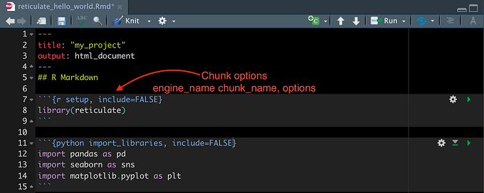
Each code chunk is delimited by three backticks at the beginning and end. Chunk options follow the opening backticks between curly brackets as pictured above. You should specify:

The engine you want to use, in our case R or Python. This is why we set the environment variable in .Rprofile earlier to point at the Python interpreter in the Conda environment created for this project. Chunks can be configured to use additional languages, for instance Bash or Perl.
(Optional) The chunk name, to hep you identify individual sections.
(Optional) Other variables to customise the functionality and output of the chunk, comma separated. Here we use include=FALSE to tell R that the code inside should be run but no output should be printed. More options are detailed here, but for now we will keep things simple.

Once you have imported the libraries as above, run the chunk. To run a code chunk, click the "play" button on the top right or use Cmd+Enter to run selected lines.

Explore and visualise the Iris dataset with Python

As an example, let's take the iris dataset built into R and visualise all its columns with seaborn. First, in an R chunk, load the data:

```{r load_data}
data("iris")
iris_df <- iris
```

Let's now use pandas to explore this data and seaborn to visualise. In a separate chunk, you can begin to write Python code natively. All Python chunks share the same environment, so the import_libraries chunk that we ran above allows us to use the respective packages throughout the document.

To "get" the iris_df object from the R environment into the Python environment, we can call it from the R environment like so r.iris_df.

```{python explore}
iris_dataset = r.iris_df
iris_dataset.head()
```
   Sepal.Length  Sepal.Width  Petal.Length  Petal.Width Species
0           5.1          3.5           1.4          0.2  setosa
1           4.9          3.0           1.4          0.2  setosa
2           4.7          3.2           1.3          0.2  setosa
3           4.6          3.1           1.5          0.2  setosa
4           5.0          3.6           1.4          0.2  setosa

Let's summarise some of these columns with pandas to decide on the right way to visualise the dataset. Let's have a look at the categorical variable in the Species column.

```{python explore}
iris_dataset["Species"].describe()
```
count        150
unique         3
top       setosa
freq          50
Name: Species, dtype: object

Awesome! There are three species in the dataset, which is not too many to visualise on the same graph. As the other columns are continuous variables, it might be interesting to see how they are distributed for each species, and how they correlate with each other. Therefore, we can use a scatterplot matrix to visualise the pairwise correlations between the continuous variables (columns one to four).

Plotting with Seaborn

Before we move on to this complex visualisation, let's first check out one of the numerical columns of the dataset with a simple boxplot:

```{python boxplot}
#summarise the column
iris_dataset["Petal.Length"].describe()
#plot boxplots with seaborn
sns.boxplot(data = iris_dataset, x = "Species", y = "Petal.Length")
plt.show()
```
count    150.000000
mean       3.758000
std        1.765298
min        1.000000
25%        1.600000
50%        4.350000
75%        5.100000
max        6.900000
Name: Petal.Length, dtype: float64

As this dataset is quite complex, a scatterplot matrix might be a better way to visualise it than a series of simple boxplots like the one above. (If you are interested in better boxplots with seaborn, check out this article.)

Let's plot the 4 x 4 scatterplot matrix using seaborn. First, we need to clear the previous plot from memory, then make the new plot.

```(python matrix}
plt.clf()
p = sns.pairplot(iris_dataset, hue="Species")
p
plt.show()
```

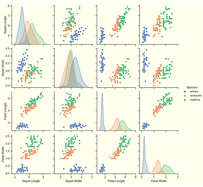
Volia! Congratulations. Now you know how to use Python in R. Conversely, to get a Python object ready to use in an R chunk, you can call it like so:

```{r}
#Python to R
py$iris_dataset
#compare with R to Python
r.iris_df
```

Final Thoughts

The Reticulate package coupled with R Markdown allows you to integrate Python code into your R workflow without switching between files and environments.
Data objects exist in separate environments for R and Python, but they get converted into the appropriate equivalent automatically when called.
It is best practice to set up Python in a virtual environment, for example using Conda like above, to control the Python interpreter used within the project as well as the libraries.

If you enjoy reading stories like these and want to support my writing, consider signing up to become a Medium member. It's $5 a month, giving you unlimited access to stories on Medium. If you sign up using my page, I'll earn a small commission. Cheers!

#r #python #programming #software-development #data-science