The HotSpot JVM is one of the most well-known JVM's (Java Virtual Machine) implementations. One of its main design objectives was to make Java applications faster.

To do this, it can gather and store different performance data metrics in a binary file called hsperfdata. This file is in a temporary directory, has the name of the process ID of the JVM instance and it's "constantly" updated. The metrics on the file track the performance of the JVM and the Java application, such as heap usage, garbage collection statistics, compilation time, thread count, class loading, and so on.

Given a copy in time of these metrics could they be quickly "analysed" by a LLM (Large Language Model) such as ChatGPT or other? And given more than one copy, in different points in time, worth analysing (e.g. before and after heavy processing), could it compare them?

Surprisingly, the answer to both questions is yes.

Feeding Java performance metrics to a LLM/ChatGPT

Let's start with how to transform the binary file into a readable format for a LLM. Let's use a tool to convert it into JSON:

$ oafp /tmp/hsperfdata_opensearch/41 in=hsperf out=pjson > data.json
$ grep Classes data.json
      "initializedClasses": "24714",
      "linkedClasses": "27501",
      "verifiedClasses": "21273",
      "defineAppClasses": "18842",
      "findClasses": "10527",
      "loadedClasses": "30565",
      "unloadedClasses": "1177",
      "sharedLoadedClasses": "1327",
      "sharedUnloadedClasses": "0"

Now let's try to feed it, with the appropriate context, to a LLM:

$ oafp /tmp/hsperfdata_opensearch/41 in=hsperf\
 llmcontext="java hsperf dump"\
 llmprompt="provide a summary of findings given the provided hsperf dump"\
 out=md

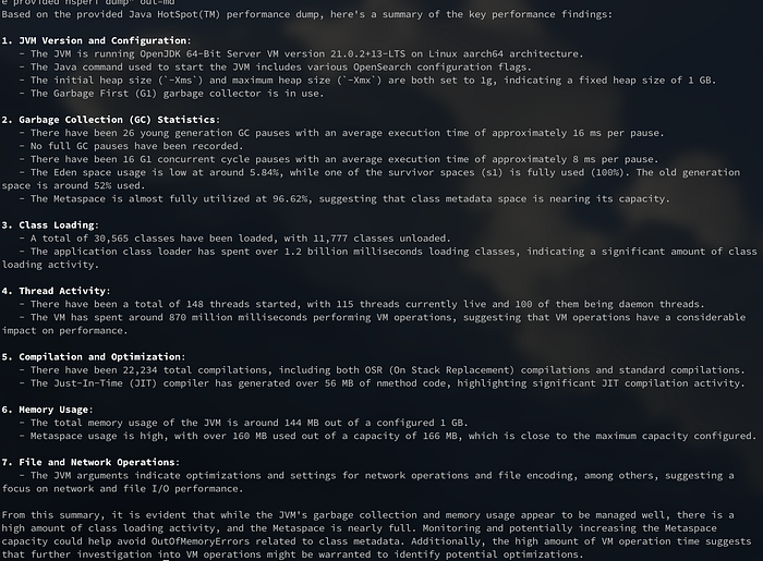
Based on the provided hsperf data, here's a summary of the performance findings:

The heap size is set to 1GB (Xms1g and Xmx1g), and the Garbage Collector (GC) used is G1GC. The heap occupancy percentage is initialized at 30% (-XX:InitiatingHeapOccupancyPercent=30). The GC reserves 25% of
the total heap size for the young generation (-XX:G1ReservePercent=25).

The JVM is using the following flags:
-Xshare:auto (enables sharing between JVMs running in the same Java Virtual Machine)
-XX:-OmitStackTraceInFastThrow (omits stack traces when fast throw is used)
-XX:+ShowCodeDetailsInExceptionMessages (shows code details in exception messages)
-Dio.netty.noUnsafe=true and -Dio.netty.noKeySetOptimization=true (disable unsafe and key set optimization in Netty library)

The JVM has loaded 30,565 classes, 1177 of which are unloaded, while 1,327 shared classes have been loaded. The total time spent by the JVM is 3,289,927,621,500 nanoseconds.

The memory usage shows a total heap size of 536 MB (536,870,912 bytes), with 144 MB (144,434,240 bytes) used and 392 MB (392,436,672 bytes) free. The meta data size is 166 MB, with 160 MB used and 5.6 MB
free.

There are no significant performance issues or warnings identified in the provided hsperf data. However, it's recommended to monitor the JVM for performance bottlenecks and memory leaks over time using tools
like Java Mission Control (JMC) or VisualVM.

It might be surprising but it wasn't necessary to use a "very large" LLM for this. This was actual produced locally by a Mistral 7B parameters model. Of course, sending it to a LLM such as GPT-4 will produce better results:

Nevertheless if there are concerns regarding sending these metrics to a public service, Mistral 7B or another larger local model might do the job for you.

Analysing two points in time

Let's try now to analyse the difference between two points in time. We are already able to transform each point into a JSON map so the natural step would be to transform it into a JSON with an array of maps. Using the "oafp" tool this is achievable by first building a NDJSON file a then converting it into a single JSON array:

# Taking a copy before processing
#
$ oafp cmd="docker exec 45 cat /tmp/hsperfdata_opensearch/41"\
 in=hsperf\
 out=json > data.ndjson
#
# After some processing...
#
$ oafp cmd="docker exec 45 cat /tmp/hsperfdata_opensearch/41"\
 in=hsperf\
 out=json >> data.ndjson

Next we will use the ndjsonjoin parameter, which instructs oafp to build the final JSON array, and feed the produced array into the LLM:

$ oafp data.ndjson in=ndjson ndjsonjoin=true\
 llmcontext="java hsperf dumps of the same application"\
 llmprompt="provide a summary of findings by comparing the provided multiple hsperf dumps considering that all of them are from the same java process"\
 out=md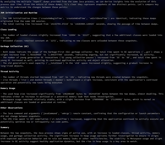

Of course, we can send more than two points in time but we should also consider the input token size available for the LLM model being used. If a LLM as a service is used input token price might also be a concern.

When analysing Java applications in remote environments you just need copies of the corresponding hsperfdata files. Usually one before and one after a specific period of processing. Nevertheless the more points in time, the better.

Want to try by yourself?

You can download the open source "oafp" tool following these instructions. It can be use directly on a docker container or by just installing it on a folder as part of the OpenAF suite. You can check all of it's options by executing "oafp -h".

Next you just need access to a compatible OpenAI API service or a local Ollama service.

You can also use the produced JSON (see commands above using "out=json") and attach the result to a GPT chat.

Configuring to use a LLM service

To configure the "oafp" tool to use a specific LLM model you just need to set the OAFP_MODEL environment variable. For example, configuring to use OpenAI's online models:

export OAFP_MODEL="(type: openai, model: gpt-4-turbo-preview, key: 'abc123', timeout: 900000)"

or using Mistral online models:

export OAFP_MODEL="(type: openai, url: 'https://api.mistral.ai', model: mistral-large-latest, key: ..., timeout: 900000)"

or using a local Ollama service:

export OAFP_MODEL="(type: ollama, url: 'https://ollama.local', model: 'mistral:7b', timeout: 900000)"

Then you can execute the "oafp" commands with the llmcontext and llmprompt parameters:

$ oafp cmd="docker exec 45 cat /tmp/hsperfdata_opensearch/41"\
 llmcontext="java hsperf dump"\
 llmprompt="provide a summary of findings given the provided hsperf dump"\
 out=md

You can also produce a HTML output instead:

$ oafp cmd="docker exec 45 cat /tmp/hsperfdata_opensearch/41"\
 llmcontext="java hsperf dump"\
 llmprompt="provide a summary of findings given the provided hsperf dump"\
 out=raw | oafp in=md out=html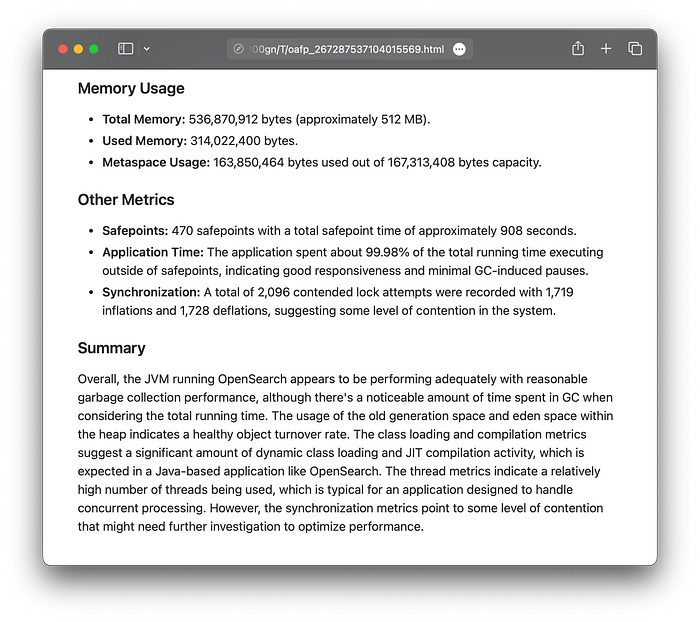

(full disclosure: I am the main author of the "oafp" / "openaf" tool)

Conclusion

Collecting multiple hsperfdata file copies, for the same application, and feeding them into a LLM model can help in the task of analysing these metrics.

As always, as with any LLM, the output needs to be careful analysed. For small LLM models, specially if they "aren't great" in reasoning the "findings" produced might be misleading and hallucinations can be expected.

Correctly used it's a helpful tool to get you a "fast start" on the analysis of the performance of a given Java process.

Mixing with other application metrics you can reach insightful results quickly, specially when comparing points in time. With periodic usage you might find some details that you might have overlook at first on a manual analyses. You will be "recalled" of those, as well as other insights, by using a LLM to assist in your analysis.