
It's a deep learning architecture which model sequential data like financial time series. It's different from Recurrent Neural Network in a way because it uses the convolutional layers, there are various advantages of using such process particularly for time-series or sequential data.
Key Components of TCN:
# The model respects the temporal order of the data by only using information from the past and current time steps when predicting the future, primarily to avoid any sought of data leakages, it's also known as Casual Convolutions.
# The important feature of this mechanism is to capture skip time series which is known as Dilated Convolutions (Spaced-Out), here we skip particular time series for example we'll skip let's say two periods so we'll look at time t=1 and time t=4 ad so on.
# In order to prevent the vanishing gradient problem and allow model to learn more complex pattern connection stabilize training by adding short cut between layers.
Advantages:
# TCN process the entire sequence in parallel which is faster to train as against the RNN.
# The combination of Dilated Convolution enables TCN to handle long memory and also incorporate the variation in data.
# The residual connection and absence of recurrence make is less prone to instability issue like vanishing gradient.
Architecture:

Maths Behind TCN:
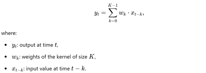
# The 1D convolution layer operator works as per below formula.
# Dilated Convolutions

# Residual Connection

# Practical Example:
We are going to train our model on SPX index for past 15 years of data. We'll use return series instead of prices as they are stationary. In terms of feature engineering we'll also use last ten days volatility and volume data as they'll help us to make prediction more accurate.
import numpy as np
import pandas as pd
import matplotlib.pyplot as plt
from sklearn.preprocessing import StandardScaler
from sklearn.model_selection import train_test_split
from tensorflow.keras import layers, models
import yfinance as yf
# === Data Preparation ===
# Simulate example data (replace this with actual SPX data)
#np.random.seed(42)
#n_days = 1000
#price = np.cumprod(1 + np.random.normal(0, 0.01, n_days)) * 1000
#volume = np.random.randint(1e6, 1e7, n_days)
# Step 1: Fetch SPX data
data_spx = yf.download("^GSPC", start="2010-01-01", end="2024-12-01")
price = data_spx['Adj Close']
volume = data_spx['Volume']
# Create a DataFrame
data = pd.DataFrame({
'Price': price,
'Volume': volume
})
# Compute returns (log returns)
data['Return'] = np.log(data['Price'] / data['Price'].shift(1))
# Compute rolling volatility (10-day window)
rolling_window = 10
data['Volatility'] = data['Return'].rolling(window=rolling_window).std()
# Log-transform volume
data['LogVolume'] = np.log(data['Volume'] + 1)
# Drop NaN values caused by rolling operations
data = data.dropna()
# Prepare features and labels
features = data[['Return', 'Volatility', 'LogVolume']].values
labels = data['Return'].shift(-10).dropna().values # Predict 10-day-ahead return
# Align features with labels
features = features[:-10]
# Standardize features
scaler = StandardScaler()
features = scaler.fit_transform(features)
# Reshape features for TCN (samples, timesteps, features)
sequence_length = 30 # Lookback window
X, y = [], []
for i in range(len(features) - sequence_length):
X.append(features[i:i + sequence_length])
y.append(labels[i + sequence_length - 1])
X, y = np.array(X), np.array(y)
# Split into train and test sets
X_train, X_test, y_train, y_test = train_test_split(X, y, test_size=0.2, random_state=42)
# === TCN Model Definition ===
# Define the TCN architecture
model = models.Sequential([
layers.Input(shape=(sequence_length, X.shape[2])),
layers.Conv1D(filters=64, kernel_size=3, dilation_rate=1, activation='relu'),
layers.Conv1D(filters=64, kernel_size=3, dilation_rate=2, activation='relu'),
layers.GlobalAveragePooling1D(),
layers.Dense(1) # Single output for next return prediction
])
# Compile the model
model.compile(optimizer='adam', loss='mse')
# === Model Training ===
# Train the model
epochs = 1000
batch_size = 32
history = model.fit(X_train, y_train, validation_data=(X_test, y_test), epochs=epochs, batch_size=batch_size)
# === Model Evaluation ===
# Predict on the test set
y_pred = model.predict(X_test)
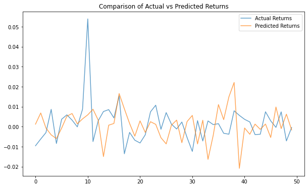
# Plot actual vs predicted returns
plt.figure(figsize=(10, 6))
plt.plot(y_test[-50:], label='Actual Returns', alpha=0.7)
plt.plot(y_pred[-50:], label='Predicted Returns', alpha=0.7)
plt.title('Comparison of Actual vs Predicted Returns')
plt.legend()
plt.show()
# === Save Model and Results ===
# Save the model
model.save("tcn_model.h5")
# Print summary
model.summary()Conclusion:
Temporal Convolutional Networks (TCNs) excel in forecasting tasks due to their ability to model long-range dependencies in time-series data effectively. Unlike traditional recurrent architectures (e.g., LSTMs or GRUs), TCNs rely on convolutional operations with dilations, which allow them to capture temporal patterns over extended time horizons without the vanishing gradient issues often encountered in recurrent models.