
Besides the title question, you might encounter the following questions in practice:
- Planning to train a 10B model — how much data is minimally required?
- Having collected 1T of data — what size of model can be trained with?
- Your boss equipes you with 100 A100 GPUs and schedules a release meeting for pretrained model in one month — how much data and what size of model would yield the best results in the given duration of time?
- Your boss isn't satisfied with the current 10B model — can you tell her/him how much improvement could be expected by scaling to 100B?
These are the questions that Scaling Laws aim to answer.
Scaling laws indicate that language model performance primarily relates to scale, rather than model architecture (e.g. width, depth). Scale mainly involves three factors: parameter count N (except embeddings), dataset size D, and computing budget C. Larger models are more sample-efficient than smaller ones, so the most computationally efficient approach is to train larger models and stop early rather than training smaller models to convergence.
The relationship between floating-point operations (FLOPs) C, model parameters N, and tokens of training D is:

Key Points
Model performance primarily depends on scale rather than architecture. Scale involves three factors: parameter count N (not including embeddings), dataset size D, and computing budget C. Model width or depth has little relation to performance.
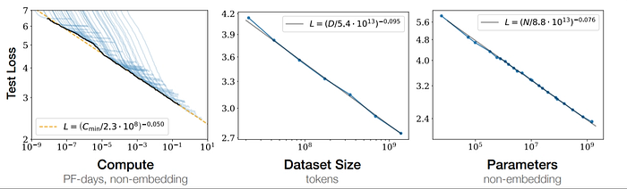
Smooth Power Laws. Performance has a power-law relationship with each of N, D, and C (when the other two are unrestricted), with trends spanning six orders of magnitude. The figure below shows that how increasing each of N, D, C leads to smooth decreases in model loss. Optimal model performance requires increasing all three factors simultaneously. The power-law relationship assumes one factor increases without constraints from the other two.
Universal Overfitting. Performance improves when N and D increase simultaneously. However, when one is fixed, increasing the other eventually yields diminishing returns. So when model size increases 8x, training data size should increase at least 5x.
Training Universality. Training curves follow predictable power-law relationships which is independent of model size. So by watching loss curves of early training stage, we can predict later loss changes.
Transfer Test Performance. When evaluating on test datasets with different distributions from training, results remain consistent but with a constant additional loss.
Sample Efficiency. Larger models are more efficient, requiring fewer optimization steps and data to achieve the same performance.
Poor Convergence Efficiency. With fixed computing budget C and unrestricted N and D, optimal performance comes from training a very large model and stopping before convergence.
Optimal Batch Size. The ideal batch size for training these models is roughly a power of the loss and can be determined by measuring gradient noise scale.
Reference: [2001.08361] Scaling Laws for Neural Language Models